Instruments and instrument properties
Adding an instrument to the measurement screen and channel assignment
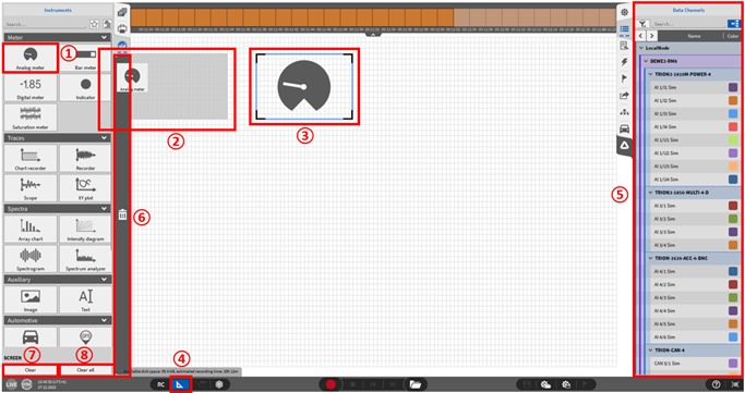
Fig. 398 Adding Instruments to the measurement screen
To add an Instrument to the measurement screen, the user must click on the Instruments menu and open it while a measurement screen is open. Select the desired Instrument by clicking on it (①), move it to the measurement screen by keeping the mouse button pressed (②) and place it wherever you like by releasing the mouse button (③). In the example of Fig. 398, an Analog meter is added to the measurement screen. The Instruments are aligned to the grey grid in the screen background. The Design mode is automatically activated when an Instrument is added to the measurement screen. The user can see that the Design mode is activated because of the blue background of the Design mode button (④) and because of the grey grid in the background of the measurement screen.
In the Design mode, the user can now change the size of the Instrument by moving the black corners of the Instrument or change the position of the Instrument by grabbing it at the blue frame.
Instrument properties - Channels tab
In the “Channel” tab, the selected data channels can be rearranged by drag and dropped. This changes the order in the label.
Deactivated channels are displayed in {} brackets and remain assigned to the instrument.
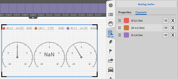
Fig. 399 Instrument properties - Channels tab, deactivated channels
Note
Several Instruments on the screen can be selected by drawing a selection rectangular with the left mouse button like it is known from Windows Explorer or similar (see Fig. 400) or by keeping CTRL+SHIFT pressed while selecting the Instruments. All Instruments on a measurement screen can be selected by pressing CTRL+A.
Fig. 400 Selection of several Instruments in the Design Mode
It is possible to activate the Design mode in the LIVE mode as well as in the REC mode and in the PLAY mode.
To assign a data channel to an Instrument, the user can select the desired channel in the Data Channel menu (⑤) by just clicking on it when the respective Instrument is selected in the measurement screen.
The functionality and properties of the individual Instruments will be explained in the following sections in detail.
As explained above, the user can add and modify the instruments on the measurement screen when the Design mode is activated. The user can also delete Instruments from the screen by selecting them and clicking on the rubbish bin (⑥) next to the Instruments menu or by grabbing the respective Instrument and move it to the rubbish bin or by selecting the Instrument and pressing the DEL-key. To exit the Design mode again, the user must click on the Design mode button and the grey grid on the background of the measurement screen will disappear. The Clear button (⑦) will erase all Instruments from the currently displayed measurement screen. The Clear All button (⑧) will erase all Instruments from all measurement screens.
Note
Pressing the Clear and the Clear all button can NOT be reverted.
Adding a whole board to an instrument via drag’n’drop instead of single channels
To add an entire measurement map to an instrument, the instrument must be placed on the measurement screen and then the map outline must be dragged into the instrument.
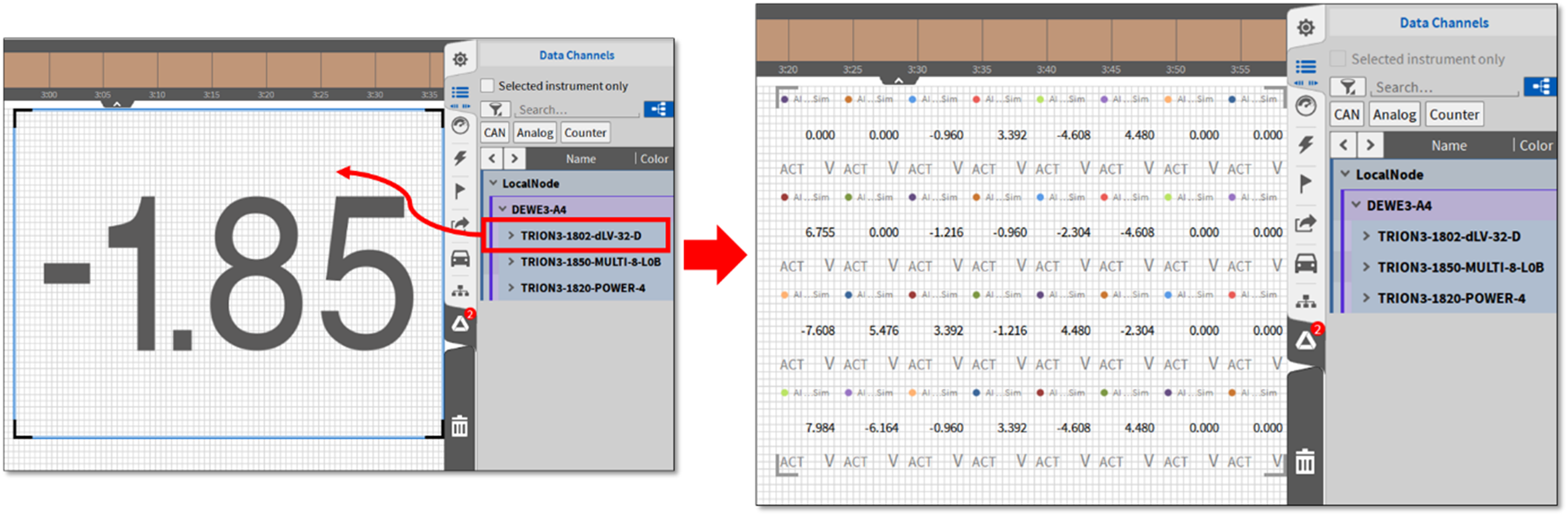
Fig. 401 Drag and drop of whole measurement board into Instrument
Several instruments can also be grouped together. Therefore, it is necessary to select all instruments which shall be grouped. Press CTRL+A on the measurement screen to select all instruments or hold CTRL and click on the instruments which shall be grouped. To group the selected instruments, click on the instrument properties button (① in Fig. 402) and click the “Group selected instruments” (② in Fig. 402) button at the bottom. This button is only visible when more than one instrument is selected.
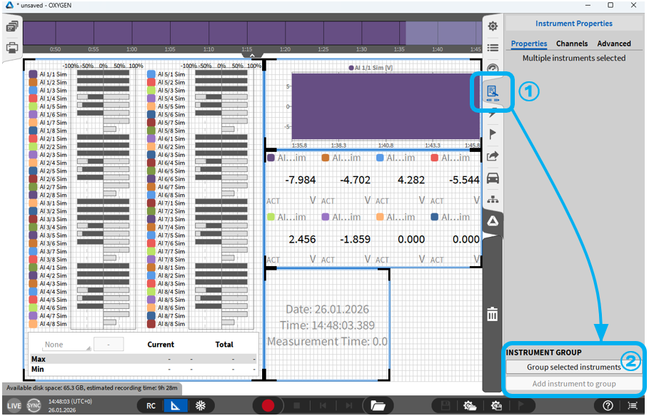
Fig. 402 Grouping of instruments
When an already created instrument group is selected and the instrument properties button will be selected (① in Fig. 403) it is possible to dismantle the selected group by clicking n the “Dismantle” Button (②in Fig. 403) .
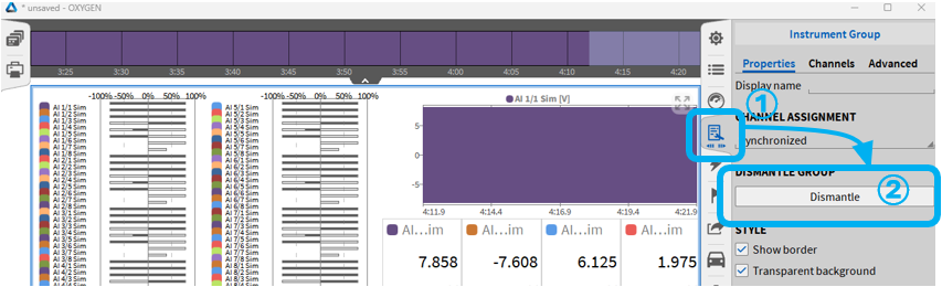
Fig. 403 Dismantle instrument groups
DejaView™
While recording data, the user is free to use the Recorder to view data from the past, even during long duration recording. This feature is called DejaView™. For activating this function, the user must click with the left mouse button in the recorder or touch the recorder with his finger and drag or swipe to the right. From this point the user is also free to pinch or scroll zoom into the data. To quickly get back to looking at the current data the user can simply press the grey >> symbol (see ② in Fig. 404) and they will be snapped back into time with the current incoming data. This is one of the most powerful features of the OXYGEN software.
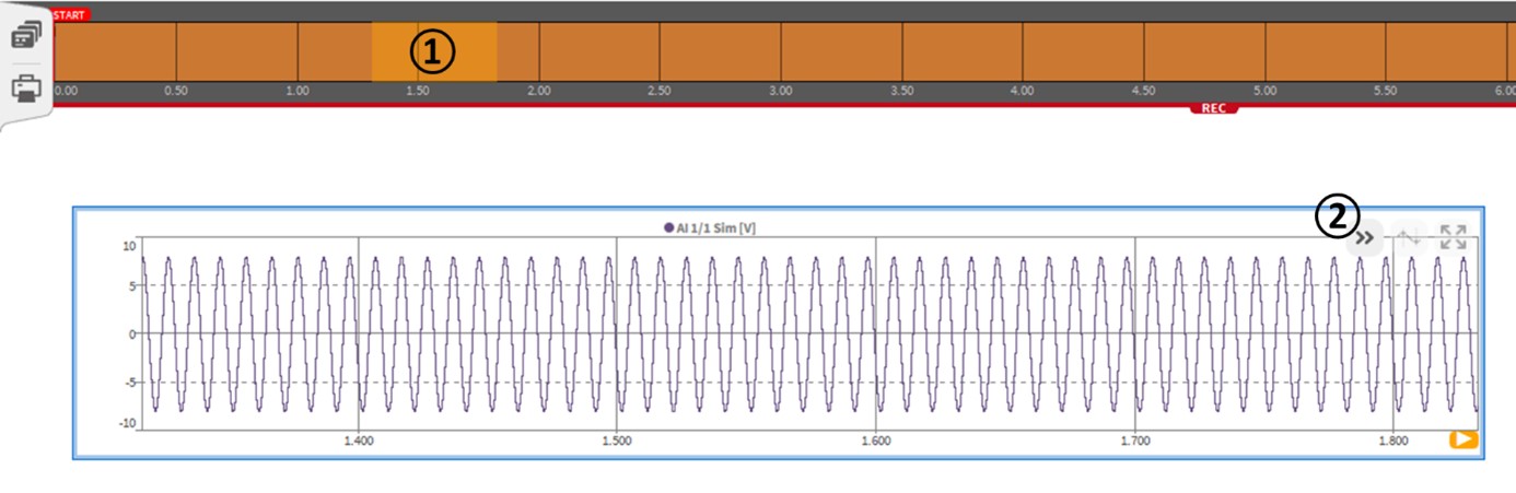
Fig. 404 Operational Features of DejaView™
Operational features of DejaView™ (see Fig. 404)
① Shows the part of the measurement file that is displayed in the recorder
② After pressing this button, the recorder will jump to the actual position of the measurement file and show the latest recorded data. A right click on this button makes the recorder show the recorded data from the recording start to the actual time position on the right end of the recorder
Note
The DejaView™ feature can be enabled and disabled in the System Settings menu point Advanced Setup (see Advanced settings).
Meters
Analog meter
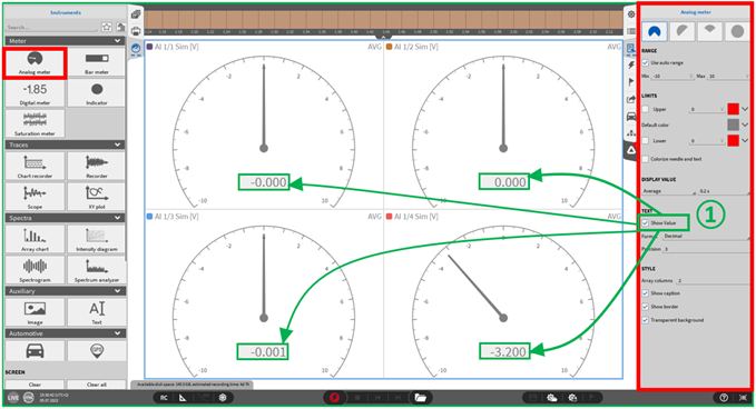
Fig. 405 Analog meter - Overview
The Analog meter can be set up in quite a few different ways. The screen capture to the right shows the various customizable Instrument Properties for this display and they are as follows:
Four different visualization options for the indicator:
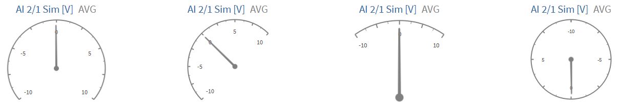
Fig. 406 Analog meter - visualization options
Range settings: The user has the options of using auto range or a user defined range.
Limits: Allows users to color the dial based on different limit values. The user also has the option to colorize the indicators needle which helps in identifying signals which have hit a limit. This is illustrated in the screen capture.
Display value: The Instruments displays either the actual channel value or the Average, RMS, ACRMS, Min, Max or Peak2Peak value at a user defined time interval of 0.1 s, 0.25 s, 0.5 s, 1.0 s, Delay, Sat (saturation).
Show value: If the checkbox for “Show value” is activated (see ① in Fig. 405), the value is additionally shown in digital form in the analog display.
Style: The user can specify the number of columns for an Analog meter cluster if several channels are selected. Selection of a transparent or untransparent background.
Show short channel name: This option does not display the node or group channel name in case the channel name has one. “AI 1/1@DEWE3-RM16” will be displayed as “AI 1/1” with the activated option.
Layer: Moves the Instrument in front of or behind another object (only applicable in Design Mode).
Note
Up to 96 channels can be assigned to one single Analog Meter.
Bar Meter
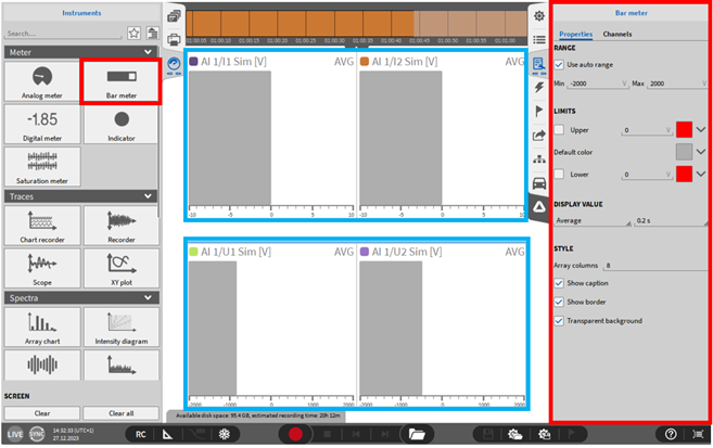
Fig. 407 Bar Meter - overview
The Bar meter is an additional tool to show the user the measurement value of a channel. The following properties are available:
Range: Allows the user to define the range of the Bar meter. There is also the option to auto range the meter based upon the input channels range setting.
Limits: Allows users to color the Bar meter fill color based on different limit values. This helps in identifying signals which have hit a limit when the display is very “busy”.
Display Value: The meter shows either the actual channel value or the Average, RMS, ACRMS, Min, Max, Peak2Peak value at a user defined time interval of 0.1 s, 0.25 s, 0.5 s, 1.0 s, Delay, Sat (saturation).
Style: The user can specify the number of columns for a Bar meter cluster if several channels are selected.
Selection of a transparent or untransparent background.
Show short channel name: This option does not display the node or group channel name in case the channel name has one. “AI 1/1@DEWE3-RM16” will be displayed as “AI 1/1” with the activated option.
Layer: Moves the Instrument in front of or behind another object (only applicable in Design Mode).
Note
Up to 96 channels can be assigned to one single Bar Meter.
Digital meter
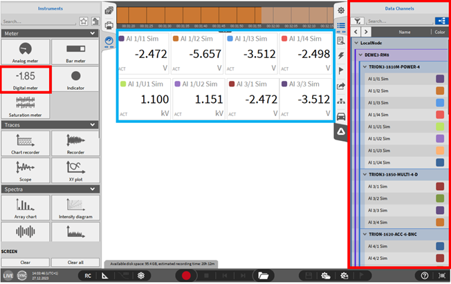
Fig. 408 Digital meter - overview
The Digital meter provides the user with the ability to definitively and quickly see what is going on with a measurement channel. This capability is further enhanced with the following list of features:
Limits: Allows users to color the Digital meters’ text based on different limit values. This really helps in identifying signals which have hit a limit when the display is very “busy”. This is illustrated in Fig. 409. It is possible to define colors for upper and lower limit as well as a default color between the upper and lower limit. First, it is necessary to define a value for the limits (except of the default setting). Afterwards it is possible to define a color for the text and the background by pressing the button ① shown in Fig. 409. When pressing one of the buttons in ① for the respective limit a new window appears (② in Fig. 409). Here it is possible to define the color for the text itself as well as the color for the background. With the buttons “Default text color” and “Default background color” it is possible to go back to the default settings, with the button “Swap” it is possible to switch the setting of the text and the background. By pressing the “Ok” button the settings will be stored for the selected digital meter.
For the background it is necessary to deactivate the “Transparent Background” option (③ in Fig. 409).
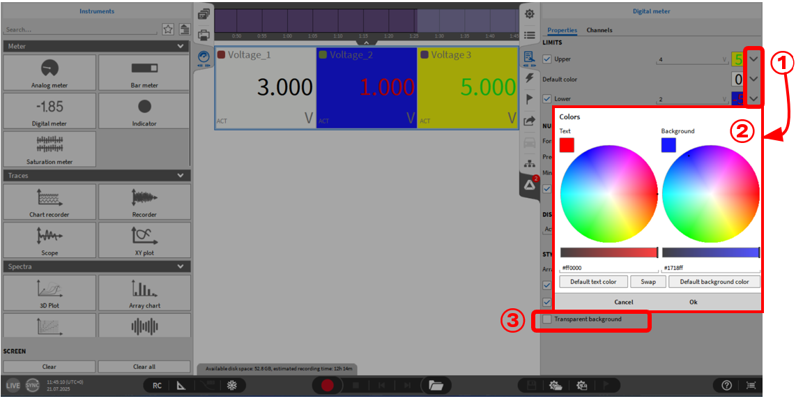
Fig. 409 Digital meter - Limits
Number Format: This option gives the ability to either display the shown values in Scientific or Decimal format.
Precision: Number of decimals right to the right of the comma can be entered here
Minimum digits: Minimum number of digits can be entered here; If the measurement value exceeds the number of digits, it will be displayed anyway but the font size will be decreased
Select suitable unit: a suitable unit prefix (i.e. milli or kilo) will be automatically selected for engineering units in case this option is selected
Display Value: The Instrument displays either the actual channel value or the Average, RMS, ACRMS, Min, Max or Peak2Peak value at a user defined time interval of 0.1 s, 0.25 s, 0.5 s, 1.0 s, Delay, Sat (saturation).
Style: The user can specify the number of columns for a Digital meter cluster if several channels are selected. Selection of a transparent or untransparent background.
Show short channel name: This option does not display the node or group channel name in case the channel name has one. “AI 1/1@DEWE3-RM16” will be displayed as “AI 1/1” with the activated option.
Show border: A grey line is drawn between the single measurement channels in case this option is selected.
Layer: Moves the Instrument in front of or behind another object (Only applicable in Design Mode).
Note
Up to 96 channels can be assigned to one single Digital Meter.
Indicator
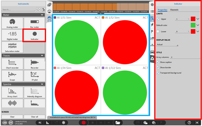
Fig. 410 Indicator – overview
The Indicator can be used for a quick status overview feedback. Depending on the current channels’ value, the Indicator changes its color. The following Indicator properties can be configured:
Limits: The user can define a default color for the indicator as well as upper and lower limit values and colors
Display Value: Assigns the Indicators’ color to the actual channel value or to the Average, RMS, ACRMS, Min, Max, Peak2Peak channel value at a user defined rate in seconds, Delay, Sat (saturation).
Style: The user can specify the number of columns for an Indicator cluster if several channels are selected
Selection of a transparent or untransparent background.
Show short channel name: This option does not display the node or group channel name in case the channel name has one. “AI 1/1@DEWE3-RM16” will be displayed as “AI 1/1” with the activated option.
Layer: Moves the Instrument in front of or behind another object (only applicable in Design Mode)
Note
Up to 96 channels can be assigned to one single Indicator.
Saturation visualization
It is possible to display the saturation visualization for selected channels. This shows the utilization (saturation) of the set measuring range for the channels displayed in the instrument in color based on the MIN/MAX value since the start of data acquisition. The saturation visualization is possible for the following instruments:
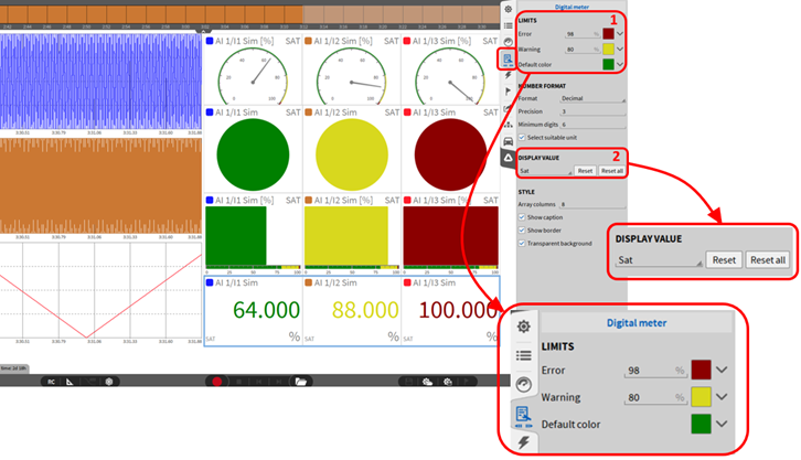
Fig. 411 Saturation visualization of channels
Analog display (see Analog meter)
Digital display (see Digital meter)
Bar graph displaymeter (see Bar Meter)
Indicator (see Indicator)
By default, the limits are set as follows:
0 … 79 %: Green
80 … 98 %: Orange
99 … 100 %: Red
After adding one of the previously listed instruments to the measurement screen, the “Sat” (saturation) mode must be selected as the display value in the settings of the respective instrument. (see ② in Fig. 411 ). By pressing the “Reset” button, the selected instrument will be reset, by pressing “Reset all”, all saturation displays will be automatically reset (instruments other than the selected instrument too). After selecting the display value “Sat”, the colors as well as the limit values for the display can be changed if required (see ① in Fig. 411).
Saturation meter
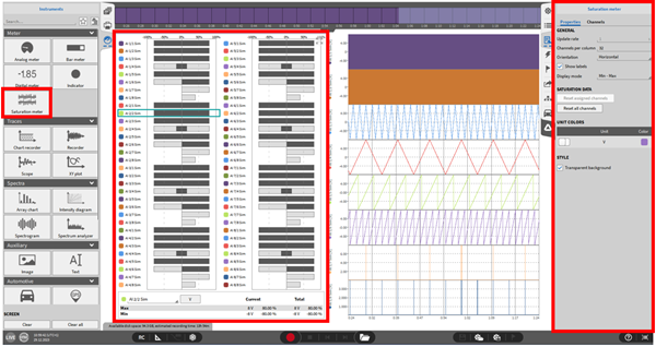
Fig. 412 Saturation Meter - Overview
It is possible to visualize the saturation of all available analogue input signals within only one instrument, the so-called saturation meter. With this instrument it is easy to see if any analogue input channel is not activated or in overload.
Fig. 413 shows how the saturation will be visualized within the instrument. The minimum and maxi-mum saturation of the channel will be displayed in light grey, whereas the minimum and maximum saturation of the channel’s latest statistics window will be displayed in dark grey. Furthermore it is possible to set different colors for the visualization of the channels with the same unit (see ⑧ in Fig. 414). Please note that the total saturation values of the channels are only available in live and recording mode and the latest statistics values can be delayed by up to one interval since the underlying calculation for the relevant data might not be available at the time of the update.
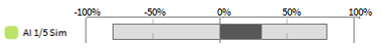
Fig. 413 Display of saturation within saturation meter
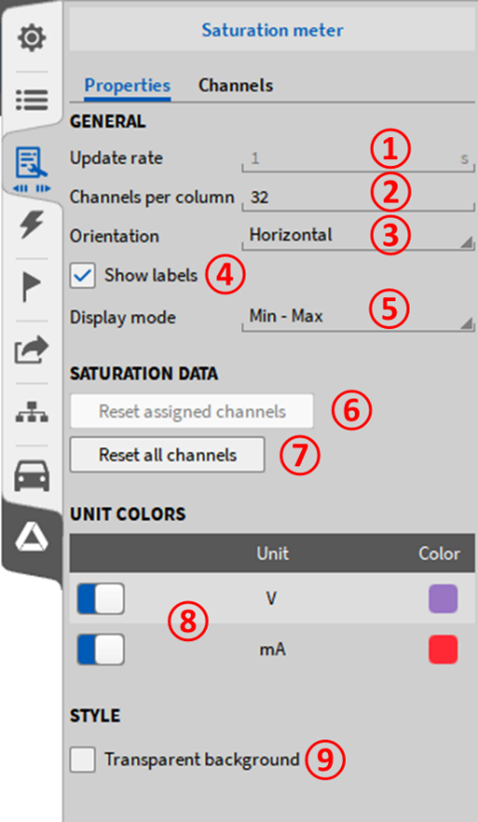
Fig. 414 Saturation meter instrument settings
No. |
Function |
Description |
|---|---|---|
1 |
Update rate |
Update rate of saturation meter. Default at 1 second and defined by statistics window in the triggered events. |
2 |
Channels per column |
Number of channels which will be displayed within one column. If the measurement systems consist, out of 128 analogue input channels and 32 will be selected, as an example, this would lead to 4 displayed columns with 32 channels each. |
3 |
Orientation |
Switch between horizontal and vertical alignment of displayed channels. |
4 |
Show labels |
Activate or deactivate the display of channel names within the saturation meter. (This is only available in the horizontal orientation.) |
5 |
Display mode |
Min – Max: Saturation will be displayed between -100 % and +100 % Zero – Max: Saturation will be displayed between 0 % and 100 % |
6 |
Reset assigned channels |
Resets the selected channels within the saturation meter. |
7 |
Format |
It is possible to assign a color to a specific unit. With the settings in Fig. 414, all channels with the unit [V] will be displayed in purple and all channels with the unit [mA] will be displayed in red. |
8 |
Precision |
It is possible to choose between “Decimal” or “Scientific” representation of the numerical display in the saturation meter. |
9 |
Unit colors |
Number of decimal places in the numerical display. It is possible to select between 0 and 20 decimal places. |
10 |
Show short channel name |
This option does not display the node or group channel name in case the channel name has one. “AI 1/1@DEWE3-RM16” will be displayed as “AI 1/1” with the activated option. |
11 |
Transparent background |
Enable or disable a transparent background with the checkbox. |
Traces
Chart Recorder
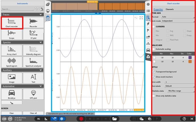
Fig. 415 Chart Recorder - overview
The Chart Recorder provides the user with the ability to view data together in one instrument as separate strip charts that are arranged one below the other. The Chart Recorder offers the same properties and analysis possibilities as the Recorder. For a detailed description refer to Recorder.
Note
Up to 16 channels can be assigned to one single Chart Recorder.
Recorder
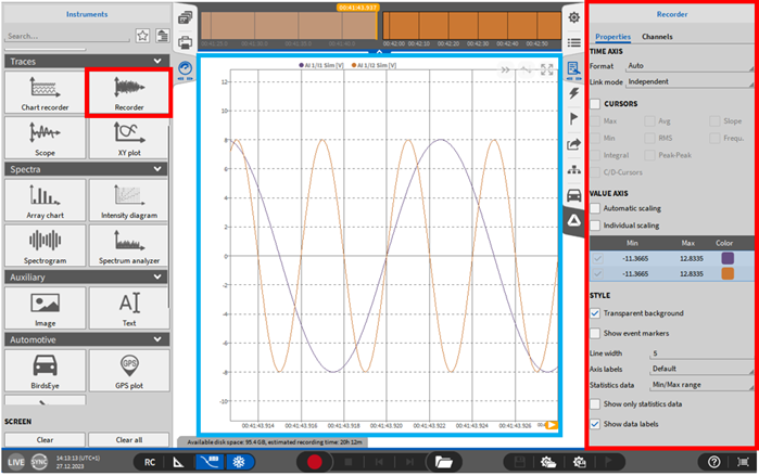
Fig. 416 Recorder - Overview
This Instrument replicates the functionality of a strip chart recorder in combination with many additional features.
Note
Up to 40 channels can be assigned to one single Recorder.
Instrument properties
The following properties can be manipulated via the Instrument Properties menu:
Time Axis: This property changes the format of the X-axis. The user can select between Auto, Absolute time and Relative time.
Auto: In Sync Mode, the Auto time format is the Absolute time, otherwise the Auto time format is the Relative time
Absolute time: The unit of the X-axis is the actual time of day set in the OS settings
Relative time: The unit of the X-axis is the relative time starting with 0:00 for every new measurement
Link mode: See Linking the time axis of several recorders.
Cursors: Select the individual parameters that are calculated when the cursors are used. For the detailed cursor description refer to section Activate cursors.
Value Axis: This property allows the user to specify the range on the Y-axis.
When the option Individual Scaling is selected, the scaling can be changed individually per channel and each channel will have an own Y-axis. If it is deselected, all channels will have one common Y-axis. For further scaling details, please refer to Quick selection Y-axis scaling.
If Automatic Scaling is selected, the Y-axis will always be adjusted to the actual displayed data.
Markers: Add up to 10 markers or remove all set markers at once. This option is only available in PLAY or Freeze mode. The markers behave similarly to the Markers. Markers can only be used when the respective checkbox is activated. If the checkbox is unchecked, the already set markers will stay but no further markers can be set without activating the checkbox again.
Style: The following properties can be adjusted:
Show short channel name: This option does not display the node or group channel name in case the channel name has one. “AI 1/1@DEWE3-RM16” will be displayed as “AI 1/1” with the activated option.
Enable/disable transparent background
Show time format
Show/hide event markers
Adjust the line width
Change the granularity of the time axis scaling via Axis labels.
Show only statistics data will solely display statistical data. The type of statistical data to be visualized can be selected via Statistics data. To display statistical data, enable statistics within the menu Triggered Events - tab Recording Mode - section Statistics. When using cursors (see Activate cursors) or markers, the displayed cursor or marker value refers to the displayed statistics data.
Show data labels hides/displays permanent data labels in PLAY mode.
Select suitable unit: a suitable unit prefix (i.e. milli or kilo) will be automatically selected if it makes sense in case this option is selected.
Label precision: Defines how much decimal places will be displayed for labels
Cursor precision: Defines how much decimal places will be displayed for cursors and markers.
Label font size: Defines the font size of labels.
Layer (only applicable in Design Mode): Moves the Instrument in front of or behind another object.
Labels
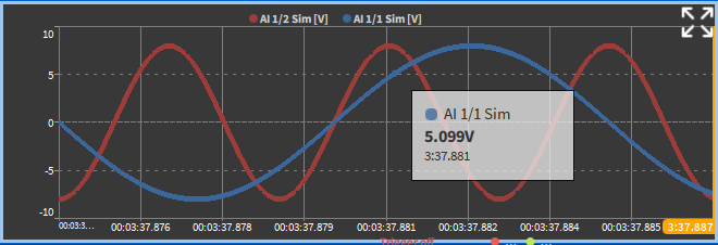
Fig. 417 Mouse-over information
To show data labels the Data Labels (see Measurement screen) button must be active.
In LIVE mode, labels appear only when the Freeze function is active and the user hovers over a data point.
In PLAY mode, clicking a data point will permanently display its label. Each permanent label can be individually positioned and removed. By unticking the Show data labels option in the instrument properties, permanent labels can be hidden. Disabling this option prevents labels from being displayed in the recorder but does not delete them.
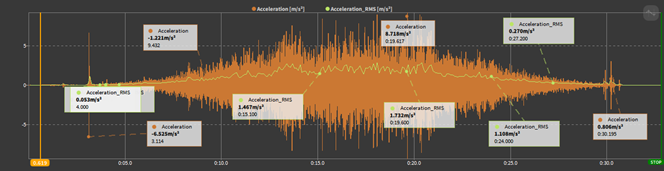
Fig. 418 Permanent labels in PLAY mode
Linking the time axis of several recorders
It is possible to link the time axis of several adjacent Recorders, the time axis of all Recorders on one page or it is possible to define Recorder groups which can also be linked over several measurement screens. This simplifies time zooming operations with several Recorders tremendously. This can be selected in the Link mode dropdown menu available in the Instrument properties (see Fig. 419) and must be selected for each Recorder separately.
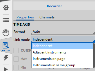
Fig. 419 Recorder link mode
When “Instruments in same group” is selected as Link Mode, there will be added an additional property to define a link group. It is possible to define any number of groups, see Fig. 420.
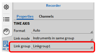
Fig. 420 Recorder link groups
The selected link mode is denoted in the lower left side of each Recorder: “Pag” for Instruments on Page and “Lnk” of Adjacent Recorders. If the link mode is set to Instruments on page “Pag”, the AB cursors are also linked for all instruments on the page.
Additional properties
To use further functionality of this instrument, the Design mode must be left. The following additional features are available:
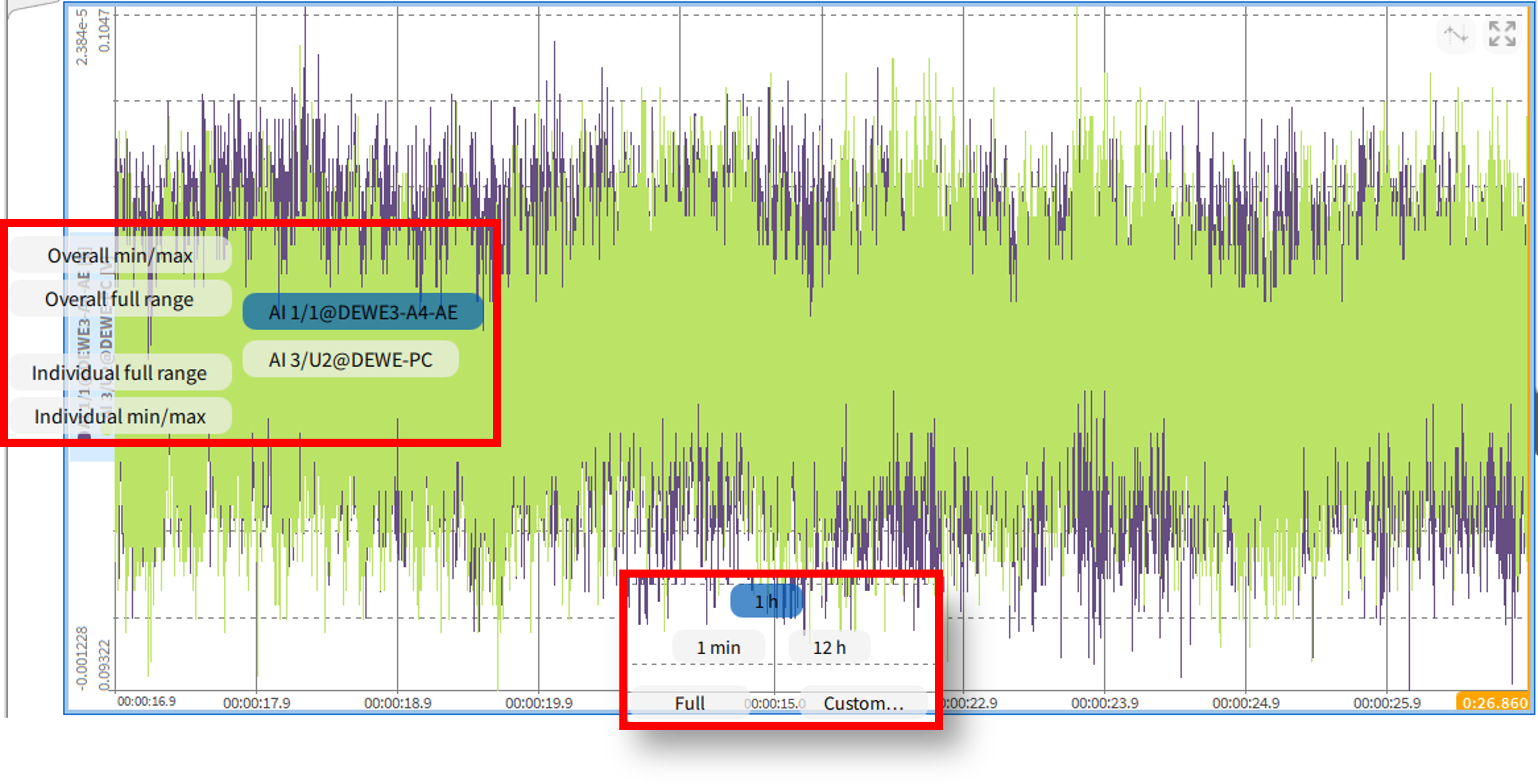
Fig. 421 Additional features of the Recorder
Pinch/Scroll zoom feature (mousewheel or right mouse button)
Quick selection X-axis scaling
This property menu appears via left click or touch and hold the X-axis of the recorder. By dragging your clicked mouse cursor or your finger into one of these menu fields and releasing you will select a new range setup. The user can select the following options:
Full: Sets the time axis of the recorder to the total elapsed recording time
Note
By one right click on the X-axis, the total elapsed recording time will be displayed as well.
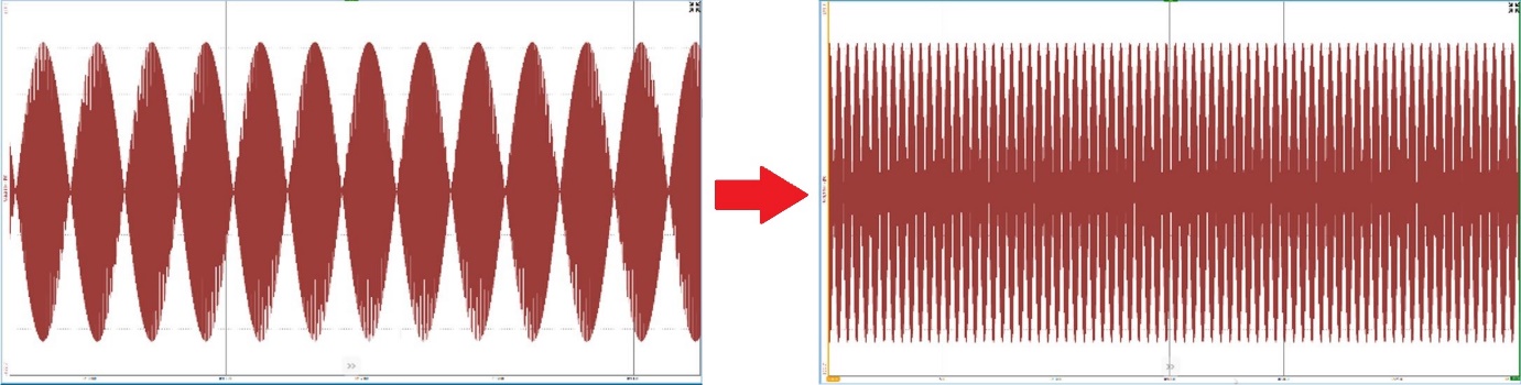
Fig. 422 Changing the X-axis scaling to the full time with one right click
1 min: Sets the time axis of the recorder to a one-minute window of the current recording time
1 h: Sets the time axis of the recorder to a one-hour window of the current recording time
12 h: Sets the time axis of the recorder to a twelve-hour window of the current recording time. If your current recording duration is below twelve hours, you will see negative time within your recorder if Relative time is selected in the Time Axis properties.
Custom: Possibility to select an individual time window:
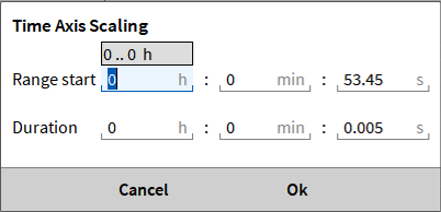
Fig. 423 Window to define a customized X-axis scaling
Useful shortcuts
Scrolling with the mouse wheel will zoom into the X-axis
Pressing the Shift key while scroll zooming will accelerate your zooming speed
Right clicking and dragging across the Recorder will allow the user to zoom into a specific region of the recorder (only available during recording or in freeze mode)
Performing a single right click will un-zoom the users Recorder instrument one step at a time
Quick selection Y-axis scaling
This property menu appears via left click or touch and hold the Y-axis of the recorder. By dragging your clicked mouse cursor or your finger into one of these menu fields and releasing, you will select a new range setup. The user can select the following options:
Overall min/max: Will set the range of all channels in the recorder to min/max value range of the highest signal amplitude displayed in the recorder
Overall full range: Sets the range of all channels in the recorder to the specified range of the channel with the highest range settings.
Note
This Scaling option is also accessible by pressing the CTRL key and clicking on a channel name.
Individual full range (Only available when Individual scaling is selected in the Instrument Properties): Sets the range of all channels assigned to the recorder to their individual full range values.
Individual min/max (Only available when Individual scaling is selected in the Instrument Properties): Sets the range of all the channels assigned to the recorder to their own individual min/max values.
A click on the individual channel name will only set the selected channel to its individual min/max value. This scaling option is also possible by clicking on the channel name on the Y-axis
Custom: (Only available when Individual scaling is not selected in the Instrument Properties): Possibility to define a customized range for the Y-axis that will affect all plotted signals:
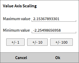
Fig. 424 Window to define a customized Y-axis scaling (Individual Scaling selected)
Example: Two channels are displayed in one Recorder. Channel 1 has a Signal Input Range of ±10 V and the range of the currently displayed data is ±8 V. Channel 2 has a Signal Input Range of ±3 V and the range of the currently displayed data is ±2 V.
Clicking on Overall min/max: The scaling of both channels is set to ±8 V
Clicking on Overall full range: The scaling of both channels is set to ±10 V.
Clicking on Individual full range: The scaling of channel 1 is set to ±10 V and the scaling of channel 2 to is set to ±3 V
Clicking on Individual min/max: The scaling of channel 1 is set to
Clicking on the name of Channel 1
will set the scaling of Channel 1 to ±8 V and not affect the scaling of Channel 2 if Individual scaling is selected
will set the scaling of the Y-axis to ±8 V if Individual scaling is de-selected
Clicking on the name of Channel 2
will set the scaling of Channel 2 to ±2 V and not affect the scaling of Channel 1 if Individual scaling is selected
will set the scaling of the Y-axis to ±2 V if Individual scaling is de-selected
Note
When Individual scaling is selected, the Custom option will not be available by clicking on the Y-axis and keeping the mouse button pressed. To enter this pop-up window when Individual scaling is selected, click on the min/max value of the Y-axis scaling:
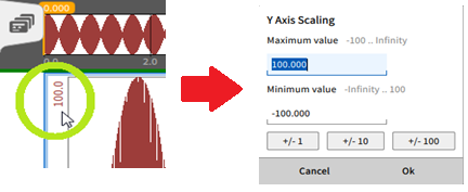
Fig. 425 Define a customized Y-axis scaling for one channel (Individual Scaling not selected)
If several channels are displayed and the scaling of all channels shall be set to the same range, click on the min/max scaling of one channel while keeping the CTRL key pressed and the scaling menu will appear as well. In this case the settings will be assigned to all displayed channels:
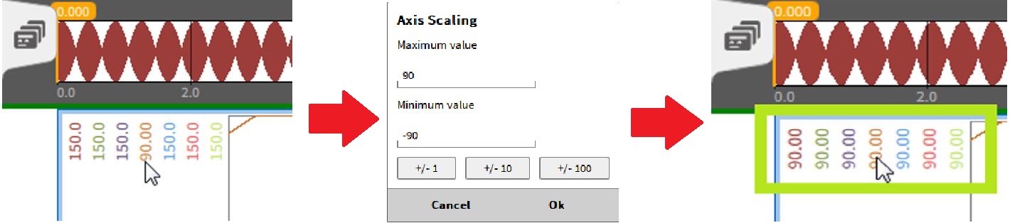
Fig. 426 Define a customized Y-axis scaling for all channels (individual scaling not selected)
Useful shortcuts
Pressing the CTRL key while scrolling with the mouse wheel will zoom into the Y-axis.
Pressing the Shift key while scroll zooming will accelerate your zooming speed
Right clicking and dragging across the Recorder will allow the user to zoom into a specific region of the recorder (only available during recording or in freeze mode and if Automatic Scaling is not selected)
Performing a single right click will un-zoom the users Recorder instrument one step at a time
Right clicking on a channel along the Y-axis will set the channels’ maximum and minimum value to the channels full range which is dictated in that channel’s setup page
Activate cursors
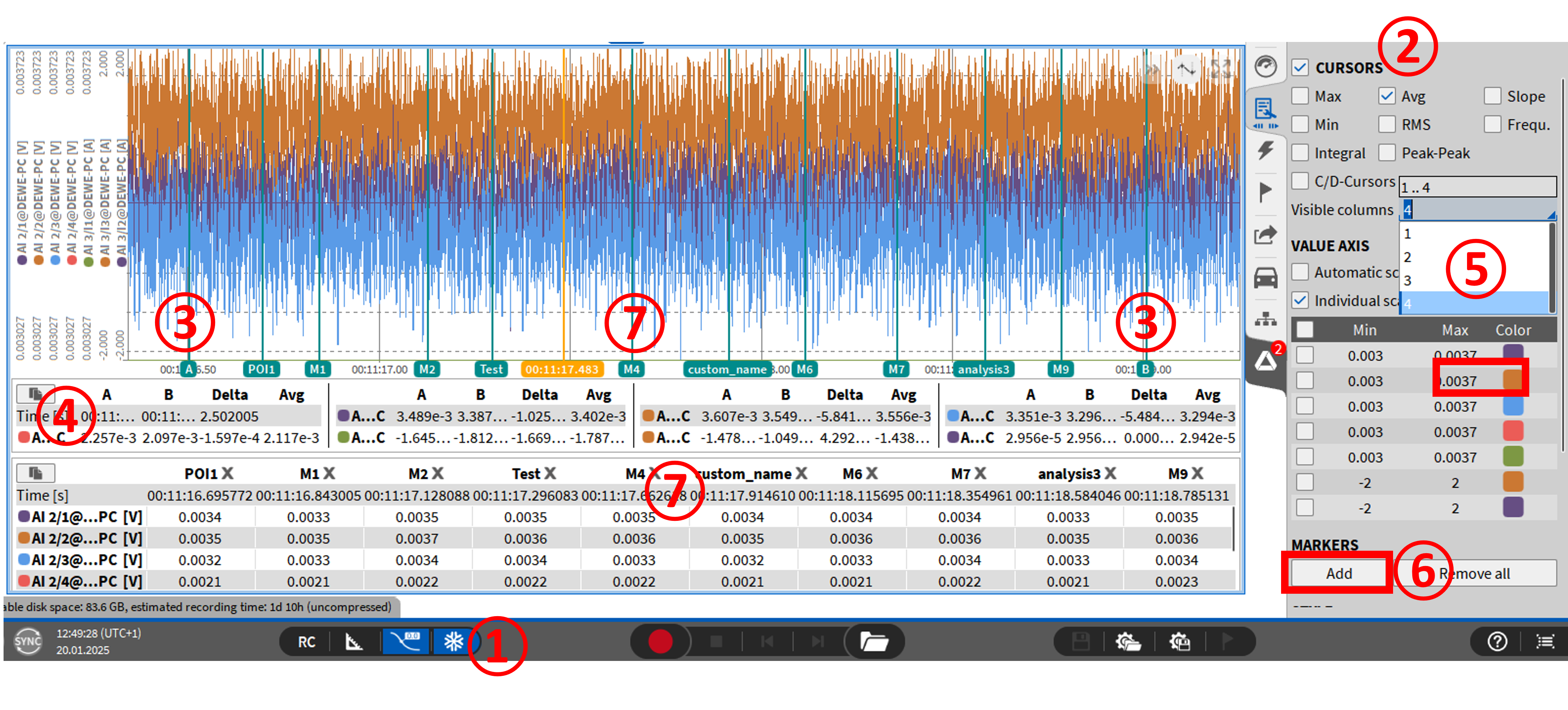
Fig. 427 Activated cursors - overview
The cursors can be activated in the upper right corner of the recorder. This option is only available in PLAY or Freeze mode. After the cursors are activated, 2 cursors A and B appear in the recorder window. It is also possible to add another AB-cursor pair (A2/B2). In addition, a table appears with the current position of the cursors, the corresponding signal value and the difference Delta between the cursor positions (see Fig. 427).

The position of the cursors can be changed by moving them to the left and right. By holding SHIFT both A and B cursor can be moved simultaneously. By default, the cursor snaps to the sample points. When holding CTRL the cursor can be moved freely between samples.
Renaming the cursors
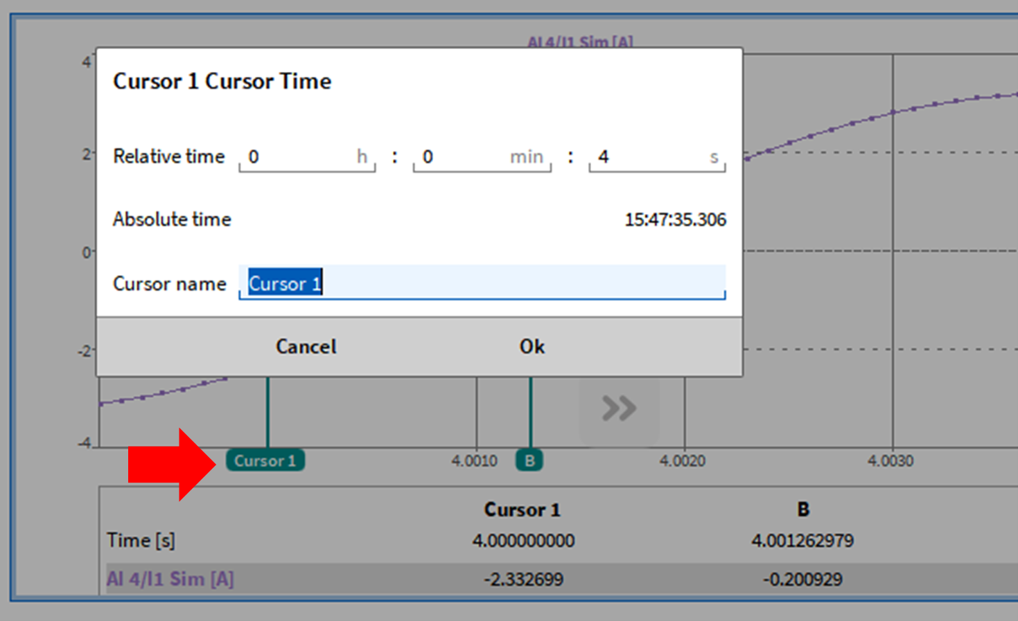
Fig. 428 Renaming the cursors
A click on the cursor name (see red arrow in Fig. 428) opens a popup with the possibility to enter a specific instant of time where the cursor shall be placed at and to change the Cursor Name. This applicable for cursor A and B. If several Recorders are used, the cursors of each Recorder can be renamed individually. If the cursors are deactivated and activated again, the individual names will be stored.
Measurement capabilities by using cursors
Additional information can be displayed in the table by selecting it in the CURSORS section in the Instrument Properties (see Fig. 427). The additional values are the following:
Max: Displays the maximum signal level between cursor A and cursor B

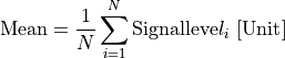
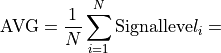
Avg: Calculates the arithmetic mean value respecting the signal level from cursor A to cursor B according to the following formula:
Slope: Calculates the slope of the signal between cursor A and cursor B according to the following formula:
Min: Displays the minimum signal level between cursor A and cursor B

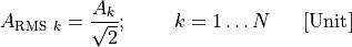
RMS: Calculates the quadratic mean value respecting the signal levels from cursor A to cursor B:
Peak-Peak: Calculates the difference between maximum and minimum signal level in range of cursor A to cursor B:

Frequ.: This value is the reciprocal value of Delta.
Integral: Calculates the area within the Y-axis and the signal from cursor A to cursor B according to the following formula:

C/D-cursors: Adds two additional cursors that can be moved vertically (not available for a Chart Recorder). Holding shift will move both cursors simultaneously.
TimeCursorA… Instant of time at position of cursor A
TimeCursorB… Instant of time at position of cursor B
Signal LevelCursorA…. Level of the signal at position of cursor A
Signal LevelCursorB…. Level of the signal at position of cursor B
Signal Leveli…. Signal level at position i between cursor A and B
i = 1…N
i = 1 =: Cursor A
i = N =: Cursor B
The following example of a 0.5 Hz sine wave that was sampled with 10 Hz will demonstrate the calculations:
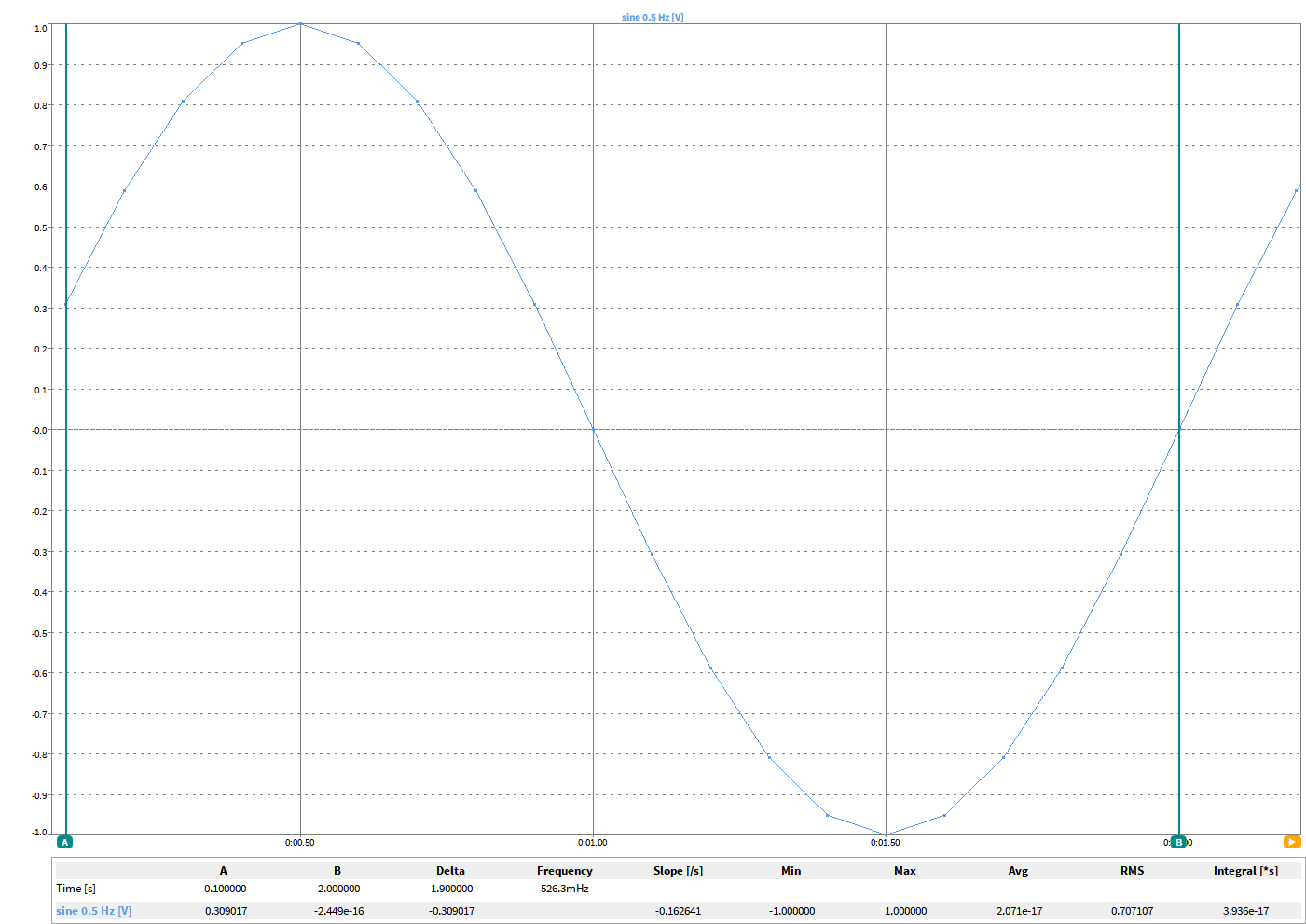
Fig. 429 0.5 Hz sine wave in a Recorder; Cursor A @ 0.1s and cursor B @ 2.0 s
In table format, the signal looks as follows:
i = 1…20; N = 20 |
Time [s] |
Sine 0.5 Hz [V] |
|
|---|---|---|---|
Cursor A |
1 |
0.1 |
0.309017 |
2 |
0.2 |
0.587785 |
|
3 |
0.3 |
0.809017 |
|
4 |
0.4 |
0.951057 |
|
5 |
0.5 |
1.000000 |
|
6 |
0.6 |
0.951057 |
|
7 |
0.7 |
0.809017 |
|
8 |
0.8 |
0.587785 |
|
9 |
0.9 |
0.309017 |
|
10 |
1.0 |
0.000000 |
|
11 |
1.1 |
-0.309017 |
|
12 |
1.2 |
-0.587785 |
|
13 |
1.3 |
-0.809017 |
|
14 |
1.4 |
-0.951057 |
|
15 |
1.5 |
-1.000000 |
|
16 |
1.6 |
-0.951057 |
|
17 |
1.7 |
-0.809017 |
|
18 |
1.8 |
-0.587785 |
|
19 |
1.9 |
-0.309017 |
|
Cursor B |
20 |
2.0 |
0.000000 |
In the following section, the values displayed with the cursors are calculated for this signal and can be compared with the OXYGEN results in Fig. 429.
Delta:

Max:
The maximum value between cursor A and B is 1.0 V @0.5s
Avg:


Slope:

Min:
The minimum value between cursor A and B is 0.0 V @1.0s and 2.0s
RMS:


Frequ.:
Integral:

Note
Besides the Recorder Instrument, the cursor option is also available for the Chart Recorder and the Scope.
Copy cursor values to clipboard
It is also possible to copy the displayed cursor values directly from the instrument in use to the clipboard and paste them into an Excel file or a simple text file, for example. To do this, simply click on the copy button displayed on the left above the table of cursor values (see ① in Fig. 430) or you can simply click in the instrument with the left mouse button and copy the values with the key combination “CTRL + C”.
Fig. 430 Copy cursor values to clipboard
Pinch/Scroll zoom feature
The zoom feature is a fundamental tool for the usage of the Recorder. It offers the user the possibility to scrutinize the data easily in real time.
Operating on a touch screen:
To perform this action with a touch screen, just do what you do with an everyday picture on your smart phone, pinch and zoom. Since the screen on a Trendcorder is so large, it is sometimes easier to use both hands to perform this action until you drill down into the finer data points.
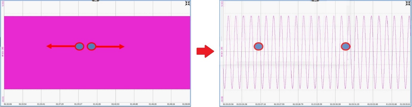
Fig. 431 Zooming on a touch screen
Operating with a mouse:
To zoom into the data with a mouse simply scroll upwards with the mouse’s scroll wheel or use the right mouse button in the following way:
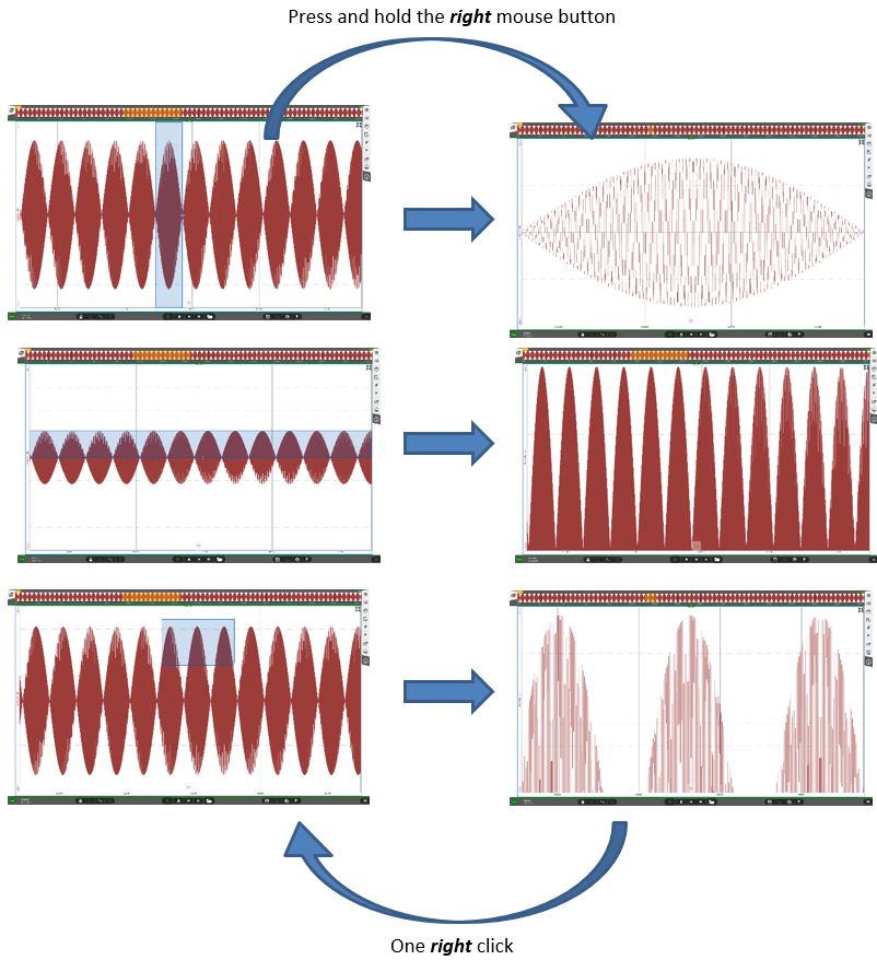
Fig. 432 Zooming with a mouse
Change settings of multiple instruments
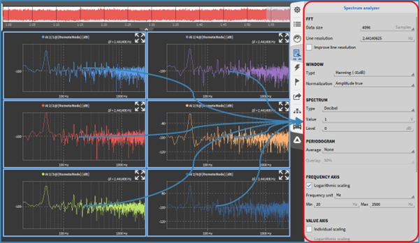
Fig. 433 Apply changes to multiple Spectrum Analyzer instruments
It is possible to change the instrument properties of multiple instruments of the same type at once. This is shown in Fig. 433 for six spectrum analyzers. Selecting multiple instruments is possible by holding the CTRL-key and clicking on different instruments successively. The combination CTRL+A will select all instruments of this measurement screen.
Scope
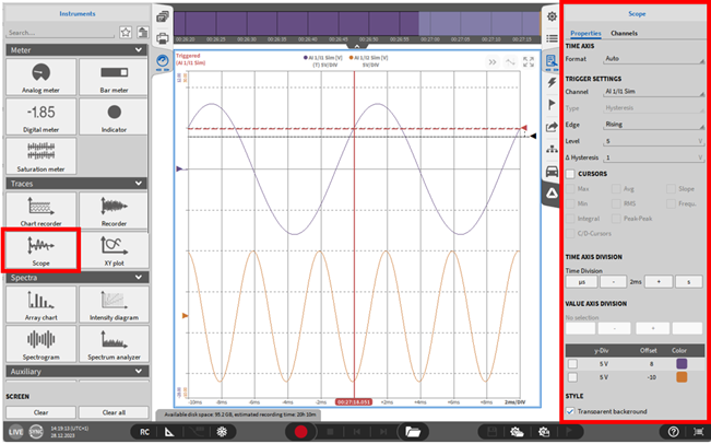
Fig. 434 Scope instrument – overview
This instrument affords the user the analysis options of a scope.
Note
Up to 8 channels can be assigned to one single scope.
Instrument properties
Trigger settings:
In the Channel selection, the user can select the trigger channel. Any channel that is displayed on the scope can be selected.
In the Edge selection, the user can select if the selected signal shall be triggered on a Rising or on a Falling edge. The difference between the two modes is shown in Fig. 435 for a 1 Hz sine wave that has an amplitude of 1.
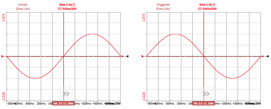
Fig. 435 Trigger on a Rising (left) and on a Falling (right) edge
In the Level selection, the user can define the level of the trigger. The level can also be set with the Level cursor (see Fig. 434) and must be within the signal range. Fig. 435 shows a 1 Hz sine wave with an amplitude of ±1 which is triggered with a rising edge (left) and a falling endge (right) on level 0 and a hysteresis of 0.5. For the rising edge this means an effective retrigger level of -0.5, and for the falling edge a retrigger level of +0.5.
In the Δ Hysteresis selection, the user can define a level the signal must pass before a new trigger event occurs. Setting a hysteresis level avoids unwanted trigger events that may occur caused by noise around the trigger level. The Δ Hysteresis level can also be set with the Hysteresis cursor (see Fig. 434).
If the signal is triggered on a Rising edge, the range of the Δ Hysteresis level can be set from [0 … (max_A + TL)].
If the signal is triggered on a Falling edge, the range of the Δ Hysteresis level can be set from [0 … (max_A – TL]].
Note
max_A: maximum signal Amplitude
TL: selected Trigger Level
Cursors: Select the desired values that shall show up when the cursors are activated. For a detailed description of the cursors refer to Activate cursors.
Time Axis Division: Change the scaling of the X-axis per division
Value Axis Division: Change the scaling of the displayed signals individually per division
Layer: Moves the Instrument in front of or behind another object (Only applicable in Design Mode)
Style:
Show short channel name: This option does not display the node or group channel name in case the channel name has one. “AI 1/1@DEWE3-RM16” will be displayed as “AI 1/1” with the activated option.
Selection of a transparent or untransparent background.
Line Width selection with default width of 1
Select suitable unit: a suitable unit prefix (i.e. milli or kilo) will be automatically selected if it makes sense in case this option is selected
Cursor precision: Limits the number of digits
Show short channel name: This option does not display the node or group channel name in case the channel name has one. “AI 1/1@DEWE3-RM16” will be displayed as “AI 1/1” with the activated option.
The Offset Cursors (see Fig. 434) can be used to displace the displayed signals vertically. Using this function will not affect the phase accuracy.
In the PLAY mode, the scope instrument can also be added or edited and has an additional trigger search functionality, meaning with the arrow keys and two arrow buttons in the instrument (see Fig. 436) jump the view to the next trigger point.
Fig. 436 Scope in PLAY mode with arrow buttons
XY plot
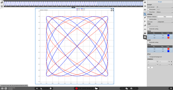
Fig. 437 XY plot instrument – overview
With the XY plot, it is possible to analyze the dependency of a measurement channel on the Y-axis to another one on the X-axis. A common application in the automotive sector is the analysis of the engine’s sound pressure level (Y-axis) in the dependency of the motor speed (X-axis). The user can adjust the following instrument properties:
XY plot
Use the X Axis Channel drop-down menu to select the channel that shall be plotted on the X-axis. Any further added channels (either via Drag-and-Drop or by clicking on them in the small data channels menu) will be plotted on the Y-axis.
Use Draw points and/or Draw lines to change the graphical characteristics of the plotted signal.
Interval
The time interval of the plotted data is displayed here and in the upper right corner of the instrument. To start the drawing of a new plot and delete the currently displayed time interval, press the Clear button.
If the check box Limit duration is selected the user can define a time interval to limit the plotted information, i.e. when 1 second is selected, all information older than 1 second will be deleted automatically.
Link mode allows users to link the time axis of instruments. See Linking the time axis of several recorders for details.
Y-axis:
Assign a user-defined min/max value to the Y-axis scaling
Individual scaling creates a separate Y-axis for each signal
Automatic scaling zooms the Y-axis to the actual displayed min and max value
X-axis:
Assign a user-defined min/max value to the X-axis scaling
Automatic scaling zooms the X-axis to the actual displayed min and max value
Reference curves:
Use the + button to create multiple reference curves as a visual boundary. These serve as guides only; no automatic action is triggered when data crosses a curve.
Click Edit to define the reference curve by entering X and Y coordinates. OXYGEN will draw linear segments between the defined points (see Fig. 438).
Note
The above-described reference curve applies solely for the XY-Plot. For the advanced math plugin Time Reference Curve, see chapter Time reference curve.
Style:
Selection of a transparent or opaque background.
Show data labels hides/displays permanent data labels in PLAY mode
Edit precision and font size of data label via Label precision and Label font size
Layer: Moves the Instrument in front of or behind another object (only applicable in Design Mode)
– Show short channel name: This option does not display the node or group channel name in case the channel name has one. “AI 1/1@DEWE3-RM16” will be displayed as “AI 1/1” with the activated option.
The Channels tab lists all pairs of channels on the X-axis and Y-axis. New pairs can be added. The X-channel and Y-channel for each plotted pair can be manually defined.
The XY Plot instrument supports A/B cursors. Unlike in recorder instruments, no statistical calculations are provided here. The cursor table displays only the current values of cursors A and B, along with their difference. Regardless of whether A/B cursors or data labels are enabled, the crosshair cursor values are always displayed in the upper-left corner of the instrument.
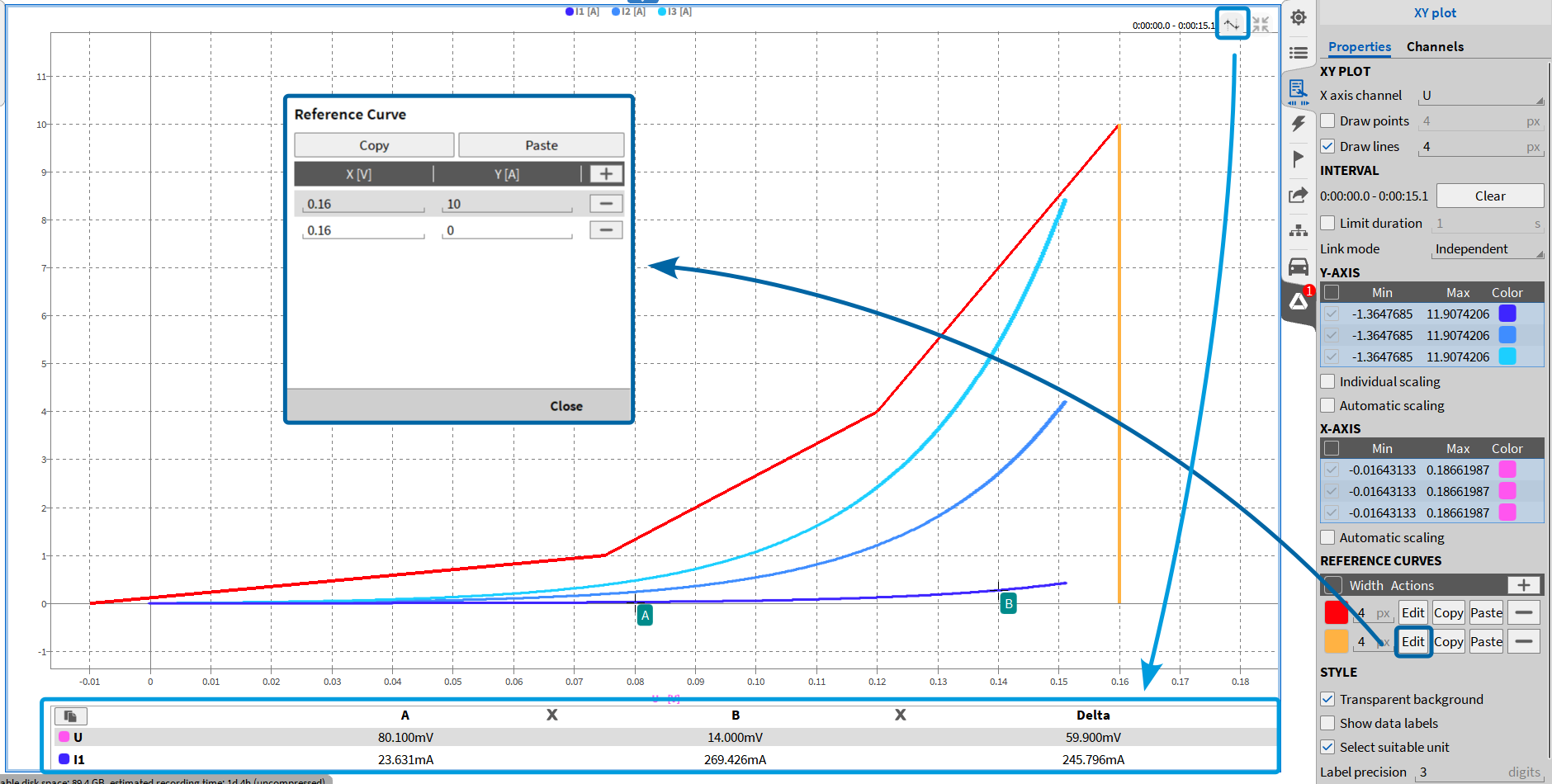
Fig. 438 XY plot – highlighted reference curve settings and A/B cursors
Note
Additional features for Y-axis scaling (see Quick selection Y-axis scaling) and zooming (see Pinch/Scroll zoom feature) are also supported in the XY-Plot Instrument
In the PLAY mode and LIVE mode (with frozen screen) the user can scroll through the measurement data by moving the orange time marker in the Overview bar or in a Recorder if one is displayed. The Interval settings in the Instrument Properties are respected during this operation.
Up to 10 channel pairs (X-channel and Y-channel) channels can be assigned to a single Table Instrument.
Spectra
3D plot
To visualize array data (3-dimensional) the 3D plot can be used. In case 2-dimensional arrays like the amplitude and phase array of the FFT are used, the 3rd dimension is the time. This plot type is useful to analyze data from the order analysis. Also, data from CPB, harmonics or the matrix sample is supported.
The instrument can be found in the spectra tab.
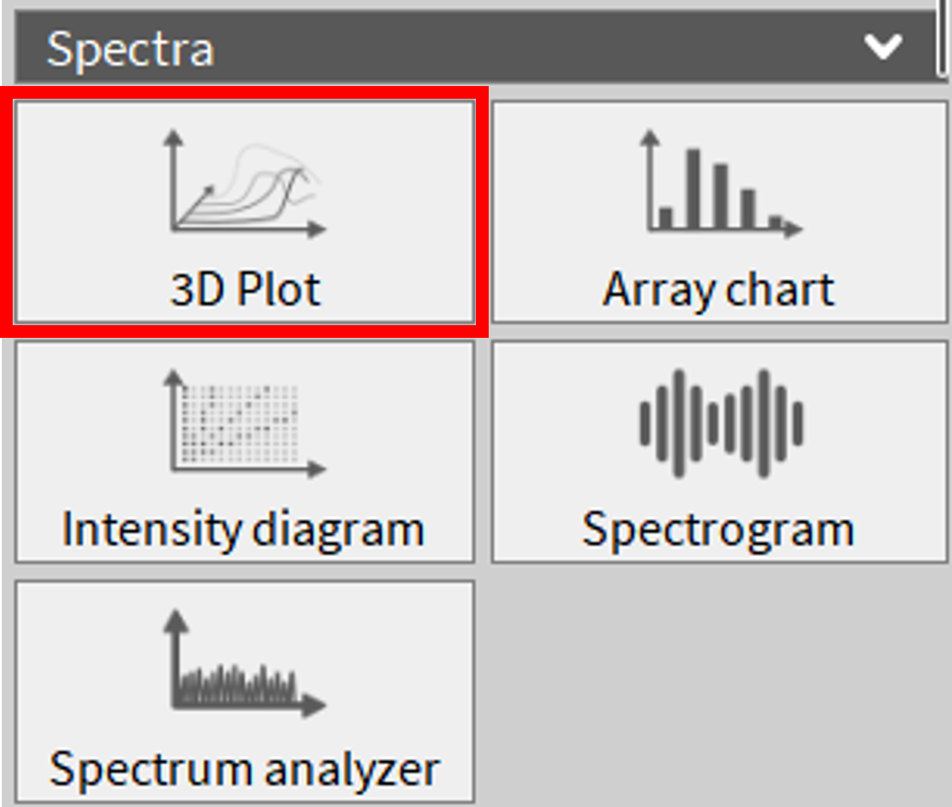
Fig. 439 3D plot instrument in Spectra tab
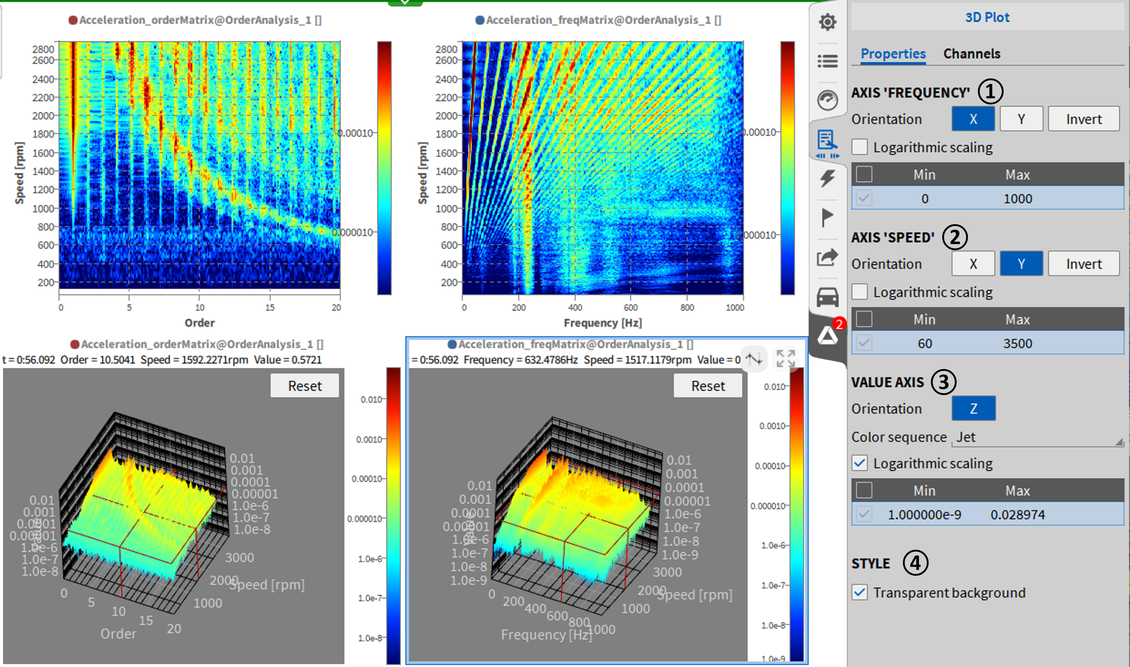
Fig. 440 3D plot example and instrument properties
No. |
Function |
Description |
|---|---|---|
1 |
Axis 1 |
Depending on the assigned channel, the first axis can be frequency, order or time. By default, the orientation of the first axis is the X-axis. This can be changed to Y or inverted. The range can be toggled as logarithmic, and the axis range can be edited manually. If the axis is a time axis, there are 2 additional properties: format and time span. Format sets the time as relative (acquisition time), absolute time. The time span determines the length of the dataset displayed in the 3d plot. |
2 |
Axis 2 |
Depending on the assigned channel, the second axis can be speed, amplitude or frequency. By default, the orientation of the second axis is the Y-axis. This can be changed to X or inverted. The range can be toggled as logarithmic, and the axis range can be edited manually. |
3 |
Value axis |
The orientation of the value axis is fixed as Z-axis. The color sequence can be chosen: RGB, Jet, Hue, Grayscale, Hot or Polar. The range can be toggled as logarithmic, and the axis range can be edited manually. |
4 |
Style |
In style the background opacity can be set to transparent. Show short channel name. This option does not display the node or group channel name in case the channel name has one. “AI 1/1@DEWE3-RM16” will be displayed as “AI 1/1” with the activated option. |
Example for first axis as time axis.
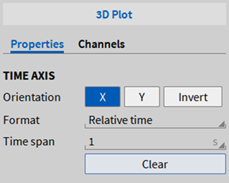
Fig. 441 3D plot with time axis
Array Chart
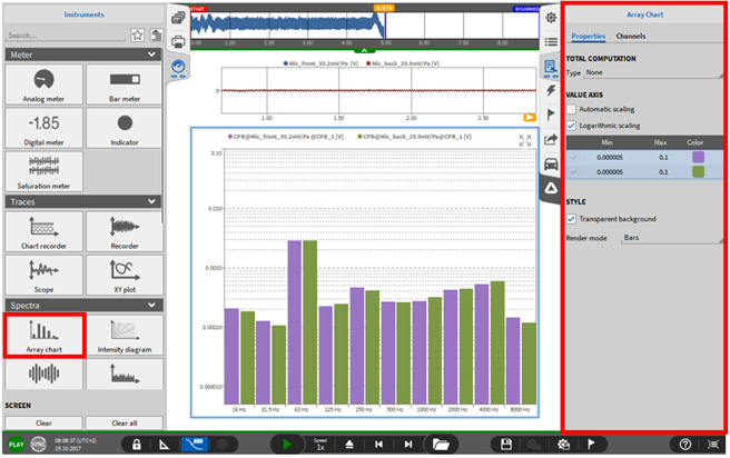
Fig. 442 Array Chart instrument – overview
The Array Chart can be used to visualize the CPB channels of a CPB (Constant Percentage Bandwidth) Analysis (refer to CPB analysis).
Note
The maximum number of channels that can be assigned to one Array Chart is two.
The Array Chart has the following Instrument Properties:
Total Computation: It is possible to include a Total column (see Fig. 443) on the right hand side that display the following value:
None: No value will be displayed
Minimum: The minimum CPB value will be displayed
Maximum: The maximum CPB value will be displayed
Energetic Sum: The energetic sum across the CPB spectrum will be displayed.
In case it is an Amplitude spectrum, the calculation is the following:
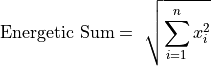
n … Number of CPB bins
xi … CPB bin with index i
In case it is a Decibel spectrum, the calculation is the following:
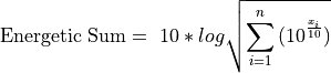
n … Number of CPB bins
xi … CPB bin with index i
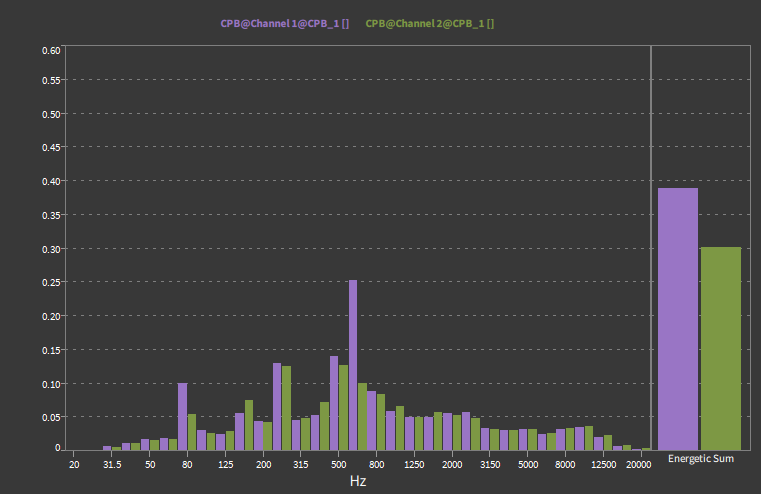
Fig. 443 Array Chart with Total column included
Value Axis: Change the upper and lower limit of the Y-axis. It is possible to choose a logarithmic scaling for the Y-axis
Style: Selection of a transparent or untransparent background.
The display mode can be selected between bars or lines (see Fig. 444).
Show short channel name. This option does not display the node or group channel name in case the channel name has one. “AI 1/1@DEWE3-RM16” will be displayed as “AI 1/1” with the activated option.
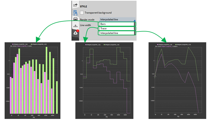
Fig. 444 Array chart instrument - bars, lines and interpolated line
Intensity Diagram
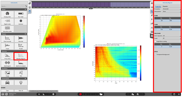
Fig. 445 Intensity Diagram instrument - overview
The Intensity Diagram can be used to display the frequency and order matrix of an order analysis channel or the resulting matrix of a matrix sampler channel, i.e. an efficiency map.
The Intensity Diagram has the following Instrument Properties:
Orientation: Horizontal orientation assigns the defined X channel to the X-axis of the instrument and Vertical orientation assigns the defined X channel to the Y-axis of the instrument.
Min/Max: the minimum and maximum value can be entered to be displayed in the instrument.
Gradient: Select a color scheme here. The color intensity can either be changed by entering the value in this menu or by moving the color bar within the instrument up or down while keeping the left mouse button pressed.
Select levels to have a more defined grading in the matrix. Select the number of levels which should be defined with a black border. The matrix on the left in Fig. 445 shows no grading and the matrix on the right has a 10-level grading.
Enter the minimum and maximum level of the color-coding
Enable logarithmic scaling by checking the checkbox.
Style: Selection of a transparent or untransparent background.
Show short channel name. This option does not display the node or group channel name in case the channel name has one. “AI 1/1@DEWE3-RM16” will be displayed as “AI 1/1” with the activated option.
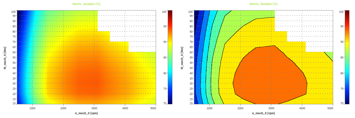
Fig. 446 Intensity Diagram of a Matrix Sampler channel without (left) and with level grading (right, 10 levels)
Spectrogram
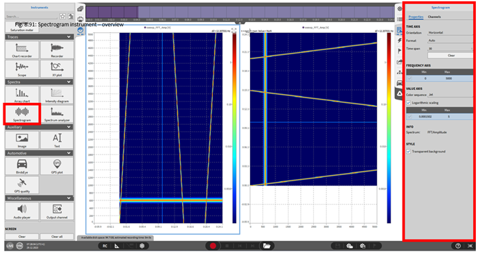
Fig. 447 Spectrogram instrument – overview
The Spectrogram may be used to display the time dependent signal trend of a FFT amplitude or phase channel that was created with the FFT math (for details, refer to FFT channels).
The elapsed time is displayed on the X-axis, the frequency on the Y-axis and the amplitude of the signal is Color-Coded to the Z-Axis (Left instrument in Fig. 447).
Note
Only 1 FFT amplitude or phase channel can be assigned to one single Spectrogram.
The Spectrogram has the following Instrument Properties:
Time Axis – Orientation: Horizontal orientation assigns the time axis to the X-axis of the instrument (see left instrument in Fig. 447) and Vertical orientation assigns the time axis to the Y-axis of the instrument (see right instrument in Fig. 447).
Time Axis - Format: This property changes the format of the X-axis. The user can select between Auto, Absolute time and Relative time.
Auto: In Sync Mode, the Auto time format is the Absolute time, otherwise the Auto time format is the Relative time.
Absolute time: The unit of the X-axis is the actual time of day set in the OS settings.
Relative time: The unit of the X-axis is the relative time starting with 0:00 for every new measurement.
Time Axis – Duration: Select the Time interval that shall be plotted on the Time Axis here. The Clear button deletes the actual displayed data from the instrument.
Frequency Axis: Select the upper and lower frequency the of the plotted data here.
Gradient: Select a color scheme here. The color intensity can either be changed by entering the value in this menu or by moving the color bar within the instrument up or down while keeping the left mouse button pressed.
Style: Selection of a transparent or untransparent background.
Show short channel name. This option does not display the node or group channel name in case the channel name has one. “AI 1/1@DEWE3-RM16” will be displayed as “AI 1/1” with the activated option.
Layer: Moves the Instrument in front of or behind another object (only applicable in Design Mode)
Spectrum analyzer
The FFT-Instrument provides the user with the ability to analyze data in real time within the frequency domain.
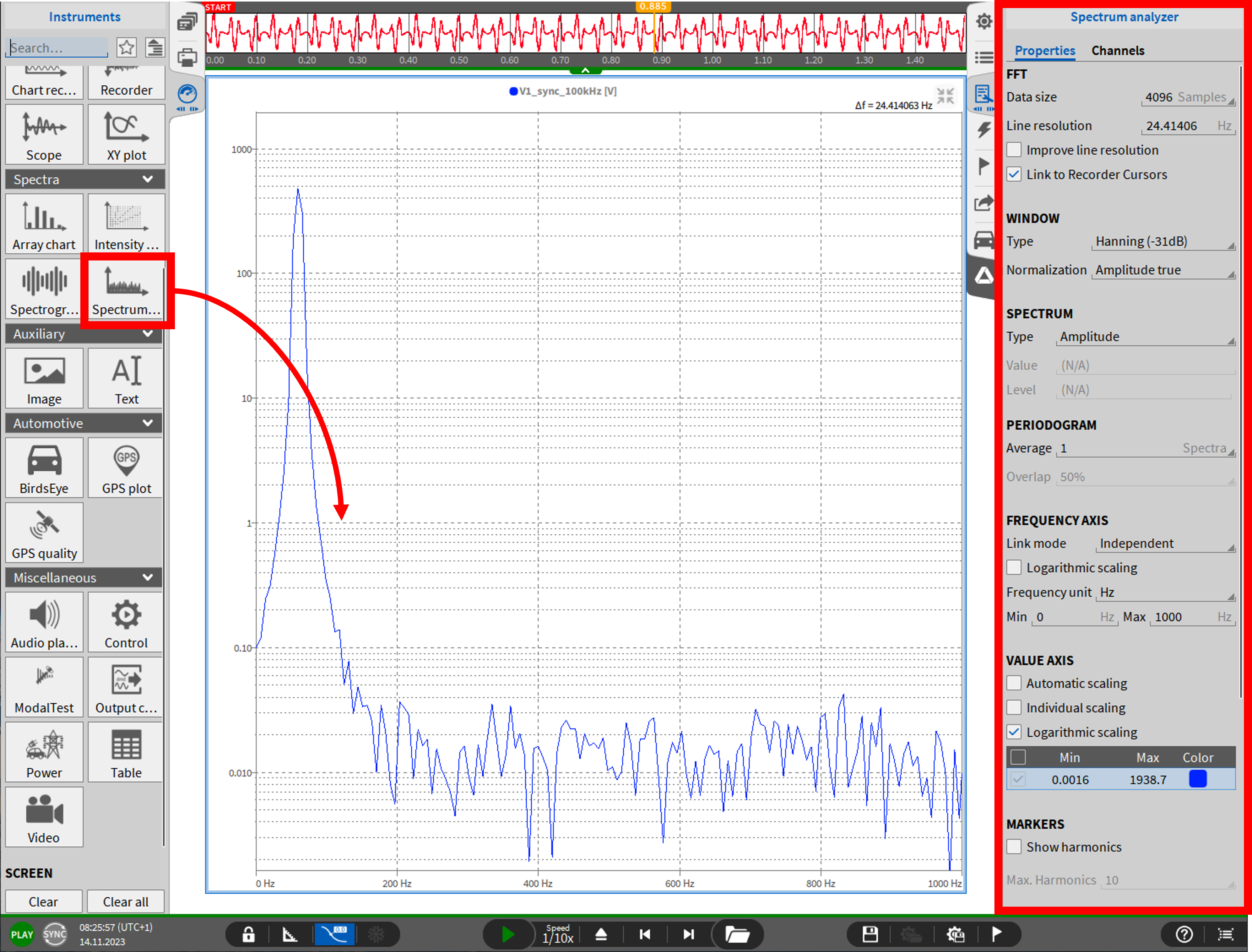
Fig. 448 Spectrum Analyzer - overview
The main properties of the instrument are FFT, Window, Spectrum, Periodogram, Frequency Axis, Value Axis, Markers, Reference curve, Style and Cross Hairs.
Both time domain and frequency domain channels can be added to the spectrum analyzer. Frequency domain channels are for example the amplitude channel created by a FFT channel from the basic math options.
Assignment of Frequency Domain Channels
Mathematical frequency channels that are calculated using the FFT math (see FFT channels) can be assigned and displayed to the Spectrum Analyzer as well. The Amplitude channel (called Channel_Name_Amp per default) and the Phase channel (called Channel_Name_Phi per default) can be assigned to the Spectrum Analyzer but no complex FFT channels (called Channel_Name_Cpx per default).
Note
Time domain channels and frequency domain channels cannot be assigned to the same Spectrum Analyzer but only to separate ones.
If frequency domain channels are assigned to the Spectrum Analyzer, the Instrument Properties are reduced to the Frequency axis and Value Axis settings (see Fig. 449). For details, refer to Additional instrument properties.
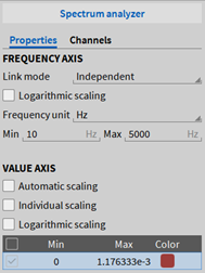
Fig. 449 Instrument Properties of the Spectrum Analyzer if Frequency Domain channels are assigned
Frequency Axis Settings
The unit of the X-axis is Hertz [Hz] per default (see ② in Fig. 450). The unit can be changed to Cycles Per Minute [CPM] which is defined as [Hz] * 60. The axis‘ minimum can be freely defined (see ③ and ④ in Fig. 450). The scaling can optionally bet set from linear to logarithmic scaling (see ① in Fig. 450).
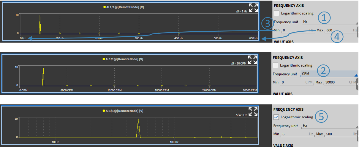
Fig. 450 Frequency axis settings
Assignment of Time Domain Channels
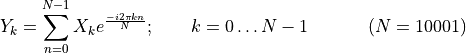
If analog channels that represent a time domain signal are assigned to the Instrument, the FFT is calculated according to the following formula:
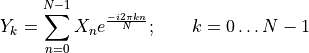
Xk… (complex) input signal
Yk… complex Fourier Transform of Xk
N… number of samples
Depending on the spectrum to be plotted, the complex Fourier Transform Yk is used for further calculations. For continuative information, refer to Section Spectrum.
Note
Up to 8 channels can be assigned to one single Spectrum analyzer.
The Spectrum analyzer provides the zooming option as well. For the detailed description of the zooming function, refer to Pinch/Scroll zoom feature.
The user can easily export the currently displayed FFT-spectrum via pressing CTRL+C and paste it into an Excel file or Notepad window
Peak Hold function: To facilitate the read off from local maxima, the user can press the SHIFT key. This makes the cursor remain at local maxima.
FFT properties for Time Domain Channels
The desired Data size (i.e. the number of samples in time domain used for the calculation of one spectrum which is denoted with N in the upper formula) can be edited here. The data size is freely definable within a range from 42 to 16777216 (224) samples. The default settings are
1024 (210), 2048 (211), 4096 (212), 8192 (213), 16384 (214), 32768 (215), 65536 (216) 131072 (217), 262144 (218), 1048576 (220), 4194304 (222) and 16777216 (224) samples.
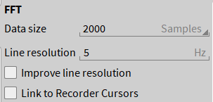
Fig. 451 FFT property of the spectrum analyzer instrument
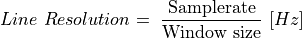
The Line resolution relates to the sample rate and the Data size:
The radio button Improve line resolution will enable zero-padding. For detailed information, refer to Additional information: improve line resolution (Enable zero-padding).
Note
If channels with different sample rates are displayed in one Spectrum analyzer:
The Line resolution is calculated for each sample rate individually and cannot be edited in the Instrument Properties. Thereby, the number of plotted FFT bins is the same for each signal but the FFT resolution is different.
Zero-padding (Improve line resolution) cannot be activated.
Note that changing the Data size will affect the Line resolution. Therefore, the line resolution is within a range from
 to
to  samples.
If Improve line resolution is de-selected, the number of calculated FFT bins is equal to the Data size. If Improve line resolution is selected, the number of calculated FFT bins is always higher than the number of data samples.
The number of plotted FFT bins is always
 . The first line is plotted @ 0 Hz and the last line is plotted @
  Hz. If logarithmic frequency axis scaling is selected, the 0 Hz line will not be plotted, because the common logarithm is not defined for 0.
Section Window
The Type and Normalization of the window function can be edited here.
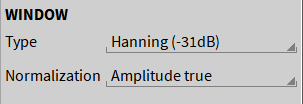
Fig. 452 Window settings for the spectrum analyzer
Window type
The Spectrum analyzer offers the usage of 7 different window functions (N denotes the Window size in samples and corresponds to the Data size):
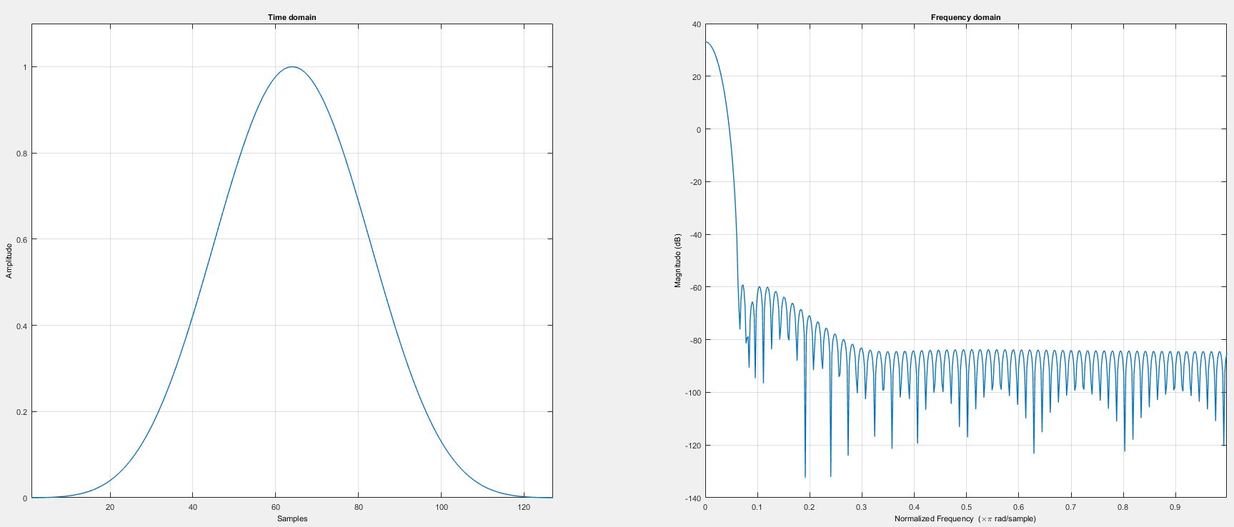
Hanning window
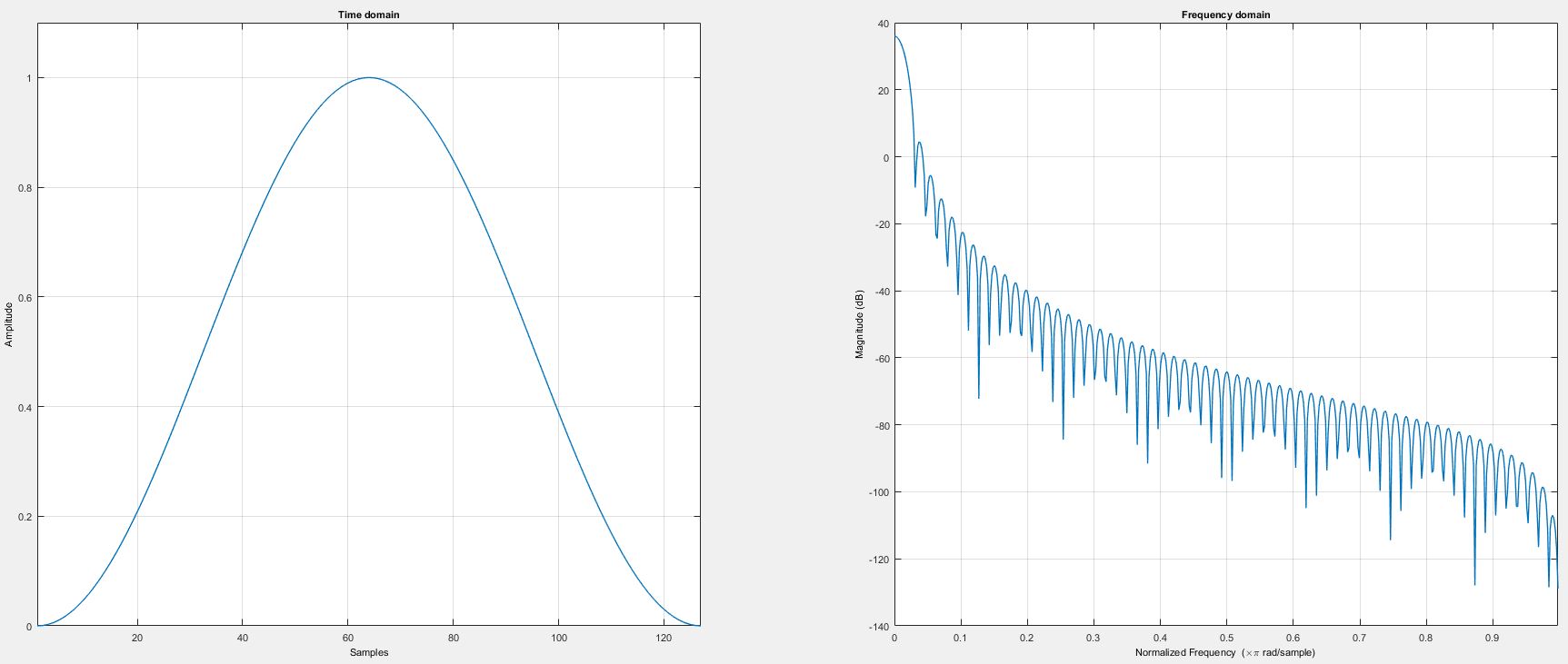
Fig. 453 Hanning window in time and frequency domain (N = 128)
Hamming window
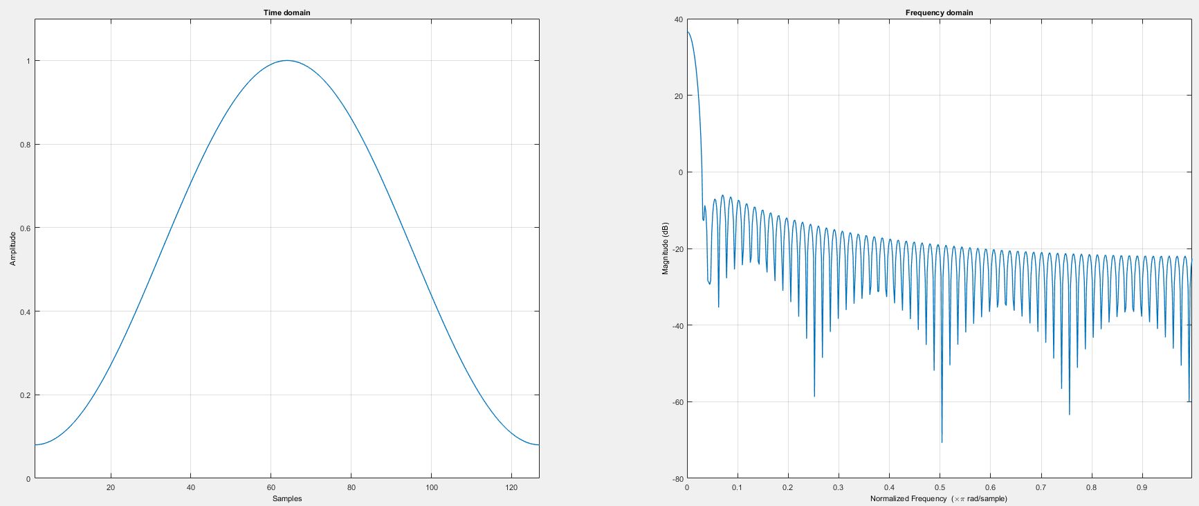
Fig. 454 Hamming window in time and frequency domain (N = 128)
α = 0.54
β… 1 - α
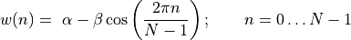
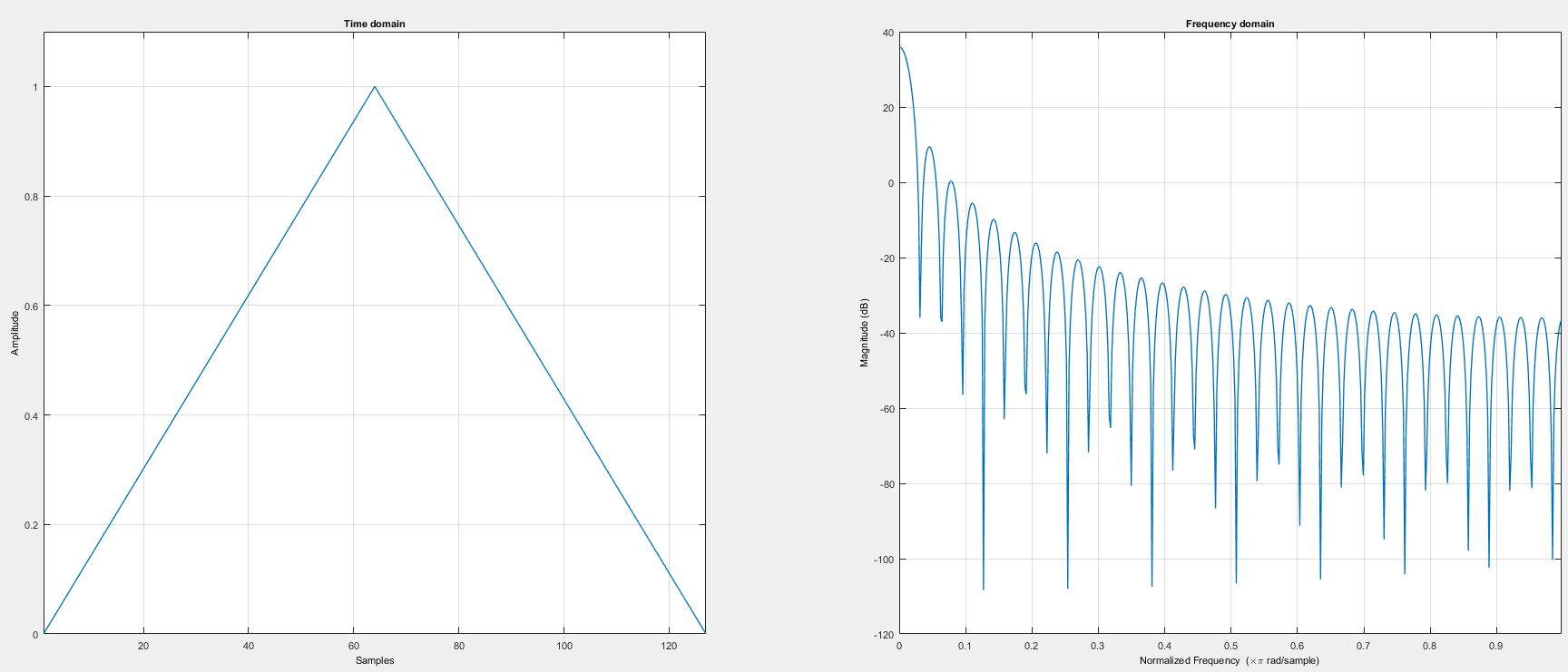
Rectangular window
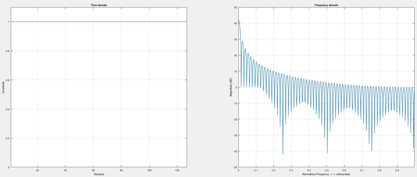
Fig. 455 Rectangular window in time and frequency domain (N = 128)

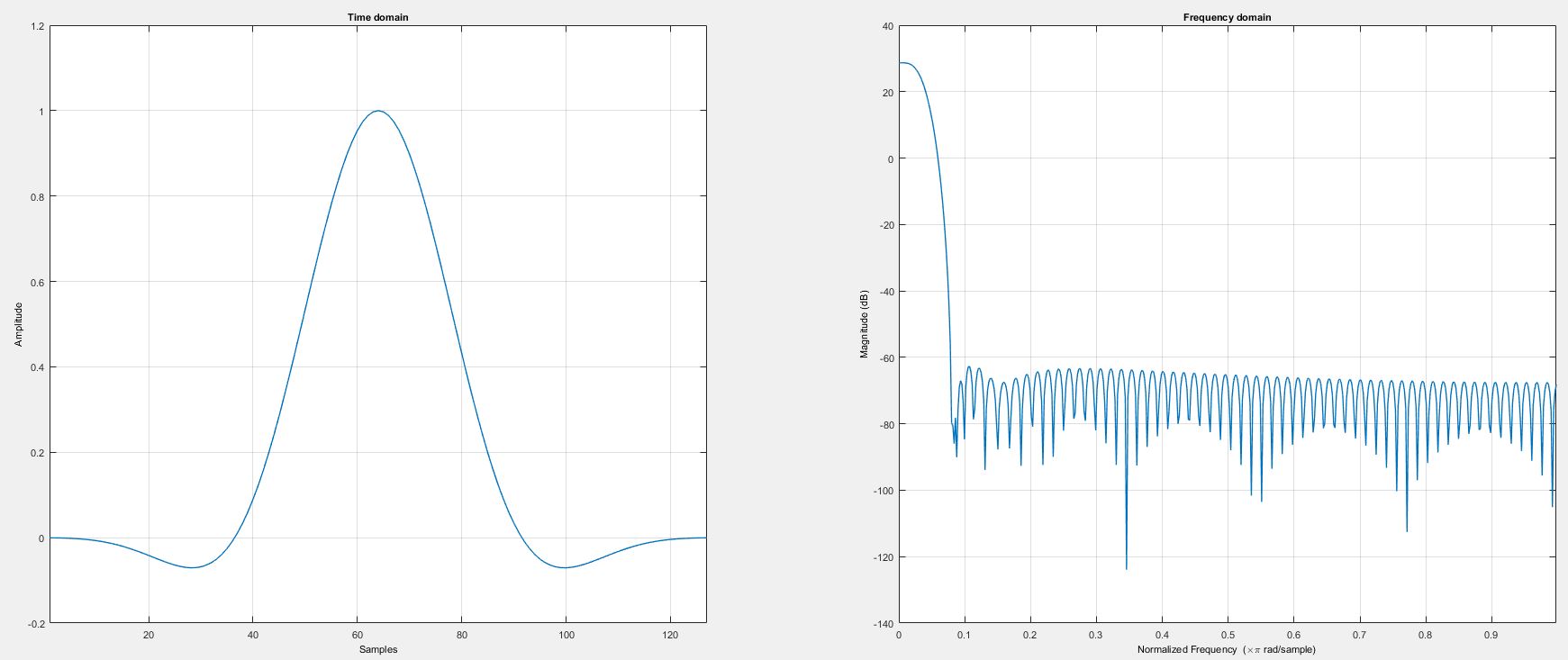
Blackman window
Fig. 456 Blackman window in time and frequency domain (N = 128)

a0 = 0.42
a1 = 0.5
a3 = 0.08
Blackman-Harris window
Blackman-Harris window in time and frequency domain (N = 128)

a0 = 0.35875
a1 = 0.48829
a2 = 0.14128
a3 = 0.01168
Flat-Top window
Flat-Top window in time and frequency domain (N = 128)

a0 = 0.21557895
a1 = 0.41663158
a2 = 0.277263158
a3 = 0.083578947
a4 = 0.006947368
Bartlett window
Bartlett window in time and frequency domain (N = 128)
The following table will give an overview and recommendations about the usage of the different window functions.
Note
This table is only a matter of recommendation and makes no claim to be complete or correct.
Signal Content |
Window |
|---|---|
Sine wave or combination of sine waves |
Hanning |
Sine wave (amplitude accuracy is important) |
Flat Top |
Narrow-band random signal (vibration data) |
Hanning |
Broadband random (white noise) |
Rectangular |
Closely spaced sine waves |
Rectangular, Hamming |
Unknown Content |
Hanning |
Accurate single tone amplitude measurements |
Flat Top |
The following figure compares the different window functions in time domain:
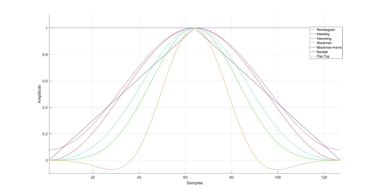
Fig. 457 Comparison of the window functions in time domain (N = 128)
The following table summarizes the two most important characteristics of the different window functions. The Main Maximum Width describes the single-sided width of the main maximum as number of FFT bins. The Main Maximum Width in Hz is the product of Main Maximum Width and Line resolution. The Max. Side Lobe Level denotes the damping of the first side lobe compared to the main maximum in decibel.
Window function |
Main Maximum Width |
Max. Side Lobe Level [dB] |
|---|---|---|
Hanning |
2 |
-31 |
Hamming |
2 |
-43 |
Rectangular |
1 |
-13 |
Blackman |
3 |
-58 |
Blackman-Harris |
4 |
-92 |
Flat-Top |
5 |
-68 |
Bartlett |
2 |
-27 |
Normalization
As the usage of a window function causes a decrement of the signals’ amplitude and power, the user can select between None, Amplitude True and Power True Normalization.
None: The spectrum will not be normalized, and the amplitude and the power error will remain
Amplitude True: The damping of the signal amplitude caused by the window function will be compensated. The power loss will remain. The correction happens according to the following formula:
Power True: The Power loss caused by the multiplication with the window function will be compensated and the amplitude error will remain. The correction happens according to the following formula:
Sk… Un-normalized signal at position k
N… Length of the Window function
Wk…Value of the window function at position k
A detailed example for the necessity to normalize FFT spectra can be found in Normalization of FFT Spectra.
Note
The normalization is applied to the signal in time domain.
Section Spectrum
In the Spectrum section, the user can select the type of spectrum plotted in the Spectrum analyzer. In the following section, the available spectra and their formula are listed.
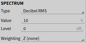
Fig. 458 Spectrum settings for the Spectrum Analyzer
Amplitude: Plots the default amplitude spectrum normalized to the number of FFT lines according to the following formula:


Amplitude RMS: Plots the RMS amplitude spectrum by dividing the Amplitude spectrum by .
Amplitude2: Plots the squared amplitude spectrum by squaring the Amplitude spectrum

Amplitude P2P: Plots Peak-2-Peak amplitude spectrum which is the amplitude spectrum normalized to the number of FFT lines multiplied by 2 according to the following formula:

For k = 0 the Peak-2-Peak amplitude spectrum is 0 per definition.
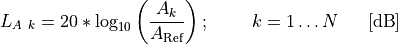
Decibel: Plots the logarithmic Amplitude spectrum referred to a freely definable reference level ARef. The reference value Aref can be edited in the Value section and its corresponding level can be defined in the Level section.
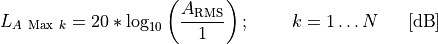
Decibel RMS: Plots the logarithmic Amplitude RMS spectrum referred to a freely definable reference level ARef. The reference value Aref can be edited in the Value section and its corresponding level can be defined in the Level section.

Decibel Max Peak: Plots the logarithmic Amplitude spectrum referred to the highest occurring value in the Amplitude spectrum. Thus, the highest occurring value corresponds to 0 dB.

Decibel V-RMS: Plots the logarithmic Amplitude spectrum referred to 1 [Signal Unit] (1 V (RMS) is a common reference level for voltage and corresponds to 0 dBV)
Decibel u-RMS: Plots the logarithmic Amplitude spectrum referred to
 [Signal Unit] (
  V (RMS) is a common reference level for voltage and corresponds to 0 dBu. 0.775V is the voltage that converts 1 mW electrical power on a 600 Ω resistance)
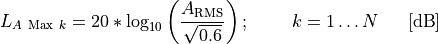
Sound Pressure Level: Plots the logarithmic Amplitude spectrum referred to 20µ [Signal Unit] (20 µPa is the common reference level for sound pressure in air and corresponds to 0 dB)

Sound Pressure Level (Water): Plots the logarithmic Amplitude spectrum referred to 1µ [Signal Unit] (1 µPa is the common reference level for sound pressure in water and corresponds to 0 dB)

PSD: The Power Spectral Density (PSD) is based on the magnitude squared spectrum (Msq) which differs from the amplitude squared spectrum (Asq) insofar that the magnitude squared spectrum is only a one-sided spectrum.


PSD-TISA: plots the Time Integrated Squared Amplitude (TISA) PSD

PSD-MSA: plots the Mean Squared Amplitude (MSA) PSD

PSD-SSA: plots the Sum Squared Amplitude (SSA) PSD

Note
PSD, PSD-TISA, PSD-MSA and PSD-SSA are different scalings of the same spectral content and differ in the physical unit.
Phase: Plots the phase spectrum from -180° … +180°.
Phase unwrapped: Plots the unwrapped phase spectrum to avoid discontinuities from -900° … +900°.
Phase radiant: Plots the phase spectrum from - … +.
Phase unwrapped (radiant): Plots the unwrapped phase spectrum to avoid discontinuities from – … +..

Weighting: allows you to apply frequency-dependent weighting to the amplitudes. The default setting is Z (none). There are also sound level weightings according to A, B, C, and D.
Section Periodogram
The usage of a window function damps the signal information at the window edges and emphasizes the signal information in the middle of the window function. If the signal is stationary, the variance of its spectrum rises. This problem can be avoided with a periodogram. If the option Periodogram is selected, the spectrum is calculated for overlapping signal parts and averaged afterwards. This procedure reduces the variance, but the spectral resolution is degraded as well.
In the Average selection, the user can select the number of spectra that shall be used for the mean value calculation. 2, 3, 4, 5, 8 or 10 spectra can be used for the mean value calculation.
In the Overlap selection, the user can select how much the single spectra used for the mean value calculation shall overlap in the time domain. The user can select an overlapping factor of 0 %, 50 %, 75 % 80 % or 90 %.
The Periodogram calculation is exemplified in Calculation of the Periodogram - Averaging of FFT windows.
Additional instrument properties
Frequency Axis: Change the scaling of the X-axis
Value Axis: Change the scaling of the Y-axis. For quick Y-axis scaling features, refer to Quick selection Y-axis scaling.
Style:
Selection of a transparent or untransparent background.
Line Width selection from 1…10
Show short channel name. This option does not display the node or group channel name in case the channel name has one. “AI 1/1@DEWE3-RM16” will be displayed as “AI 1/1” with the activated option.
Layer: Moves the Instrument in front of or behind another object
Note
The properties of the FFT can be changed and updated in the PLAY mode as well as in the LIVE and REC mode.
Markers
Fig. 459 FFT Marker - Overview
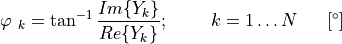
To analyze the behavior of a certain frequency line, the user can display the actual value in a table below the FFT plot. Therefore, the user must activate MARKERS with the respective checkbox in the instrument settings and select the desired frequency line with a mouse click afterwards. Then, the selected point will show up in the table. The user can change the frequency position by moving the respective cursor across the frequency axis or with a double click on the frequency in the table. Up to five frequency lines can be displayed in the table simultaneously. While moving the mouse in the frequency plot, the actual frequency and the actual signal value of the signal next to the cursor are displayed in the upper left corner. When markers are set and the respective checkbox in the instrument settings will be deactivated, the set markers stays untouched, but it is not possible to add new markers until the MARKERS checkbox will be activated again.
Usage Of Harmonics Cursors
Harmonics Cursors can be displayed by checking Show Harmonics (see ① in Fig. 460). The number of harmonics can be set from 1 to 10 (see ② in Fig. 460). Harmonics are marked with cursors (see ③ in Fig. 460) and the harmonics amplitude is displayed at the instrument‘s bottom (see ④ in Fig. 460).
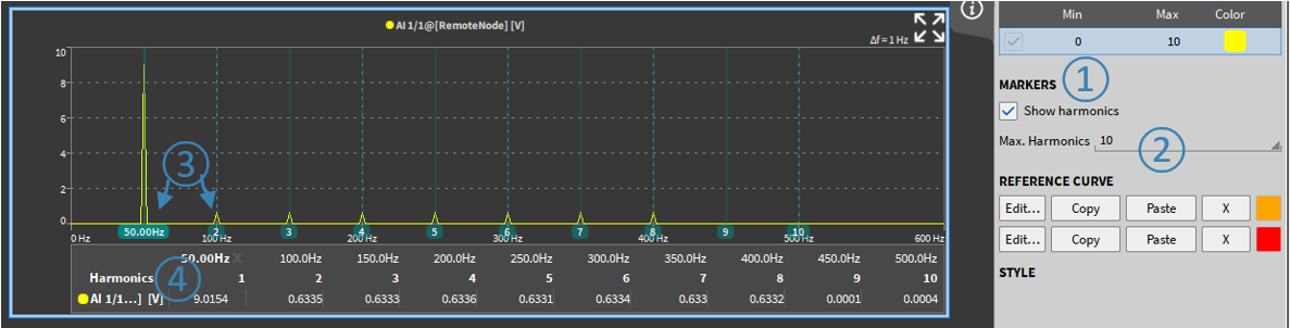
Fig. 460 Usage of Harmonics Cursors
The cursor position can be changed by entering a new frequency for the first harmonic (see ⑤ in Fig. 461). It is also possible to move the first harmonic cursor with the left mouse button (see ⑥ in Fig. 461). The position of the higher harmonics is automatically adjusted.
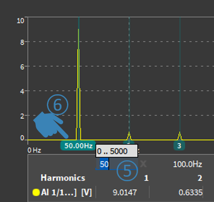
Fig. 461 Changing the 1st Harmonics cursor position
Reference Curves for the Spectrum Analyzer
The Spectrum Analyzer provides the possibility to create reference curves for threshold monitoring in the frequency domain.
An orange and a red colored reference curves can be created which will colorize the instruments’ background orange or re if the signal exceeds the reference curve.
The red reference curve has a higher priority than the orange one. This means that the instruments’ background will be colored red if the threshold of both reference curves will be exceeded. The colored background will be reset automatically when the threshold is decreased again.
To create a Reference curve, press the Add.. button in the Reference Curve section of the Spectrum Analyzers’ Instrument Properties (see Fig. 462). If the Linear interpolation checkbox is enabled, the set X and Y values are interpolated.
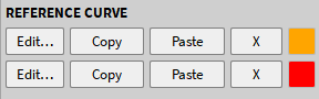
Fig. 462 Instrument properties for Reference curves
A popup menu will open and the reference curve can be set up in table form (see Fig. 463). The + button can be used to add a value. If the Linear interpolation checkbox is enabled, the set X and Y values are interpolated.
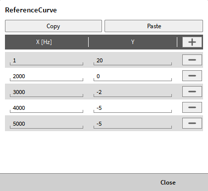
Fig. 463 Table for reference curves definition
The following Fig. 464 and Fig. 465 demonstrate the steps to create an orange and a red reference curve:
Click on the Edit… button
Press + to add one or more lines to the table
Enter the frequency and the corresponding reference value to the table
Press Close when finished and the curve will instantly be displayed
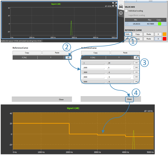
Fig. 464 How to create an orange reference curve
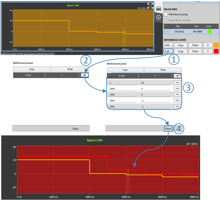
Fig. 465 How to create a red reference curve
The Copy and Paste buttons can be used to copy and paste the table from the orange to the red curve and vice versa (see Fig. 466) or to export and import a value table into / to clipboard for interacting with Excel or other 3rd party software (see Fig. 467).
The X button (see Fig. 462) can be used to delete a reference curve again.
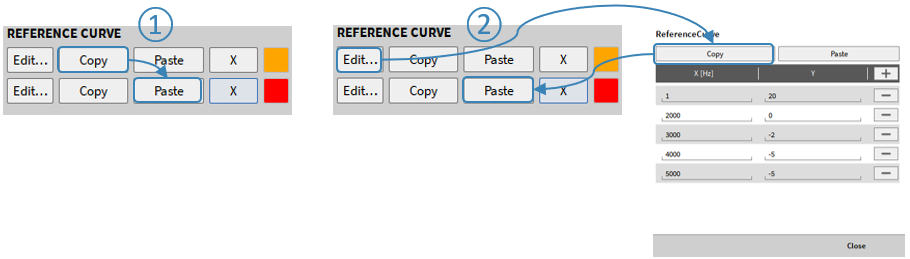
Fig. 466 Copy and paste settings from one reference curve to another
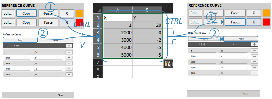
Fig. 467 Copy and paste values from/into Excel
As soon as the table has been set up, the reference curve will be displayed in the Spectrum Analyzer (see Fig. 468, Fig. 469 and Fig. 470).
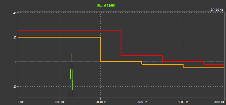
Fig. 468 Reference curves without limit exceeded
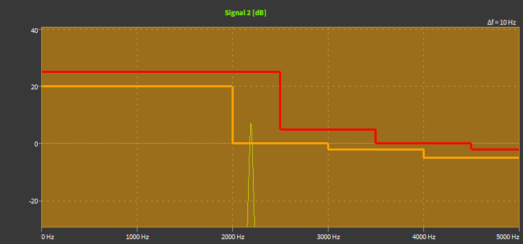
Fig. 469 Reference curves with orange limit exceeded
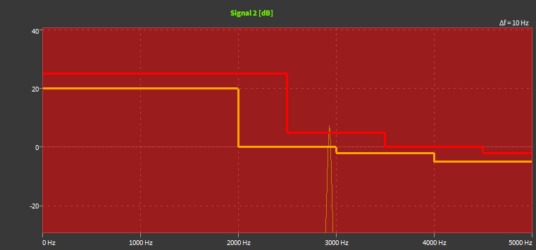
Fig. 470 Reference curves with orange and red limit exceeded
Cross hairs
There are 2 options for crosshairs: Use crosshair cursor and Use peak cross hair. Additionally the Line width of the cross hair can be defined.
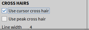
Fig. 471 Cross hairs option of the spectrum analyzer
With the “Follow Peak” function at the Crosshairs option, the peak value in the visible area of the FFT instrument is visually marked with the help of a crosshair (see Fig. 472). The cross hairs jumps automatically to the highest peak, which makes it easy to recognize.
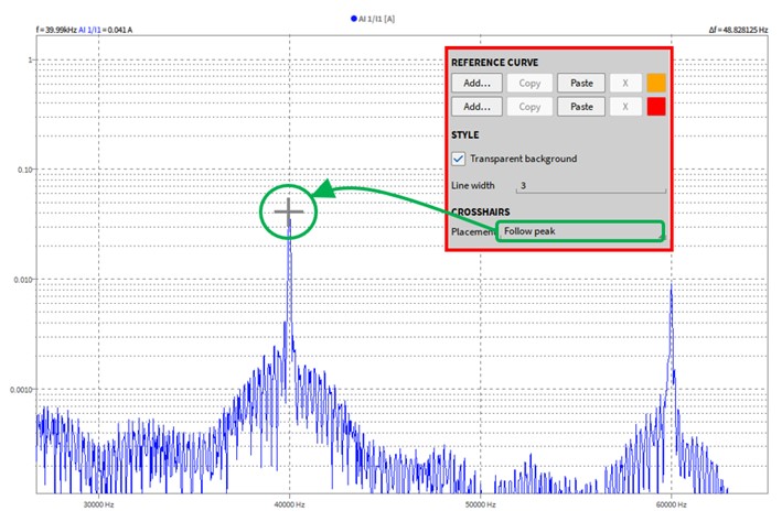
Fig. 472 Follow Peak
FFT for recorder region
It is also possible to calculate the FFT for the assigned time domain channel based on a selection from A/B cursor in a recorder. For this to work, the recorder needs to be on the same page and has its settings to “Link mode: Instruments on page” (①). The channel of the recorder must be also assigned to the spectrum analyzer and the FFT option “Link to Recorder Cursor” must be enabled (②).
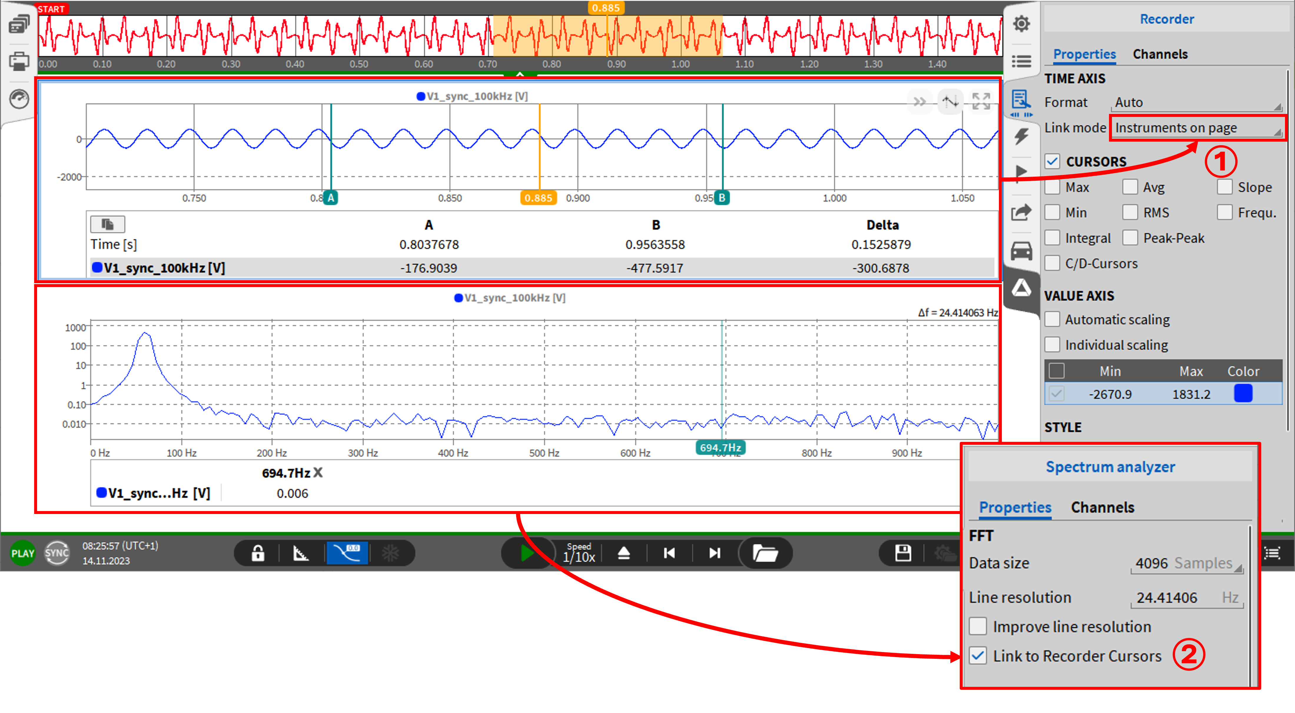
Fig. 473 Spectrum analyzer with data based on recorder region
This function is available in LIVE (freeze) and PLAY mode.
Additional information for the spectrum analyzer properties
Further explanations on line resolution, normalization, and averaging are provided below.
Additional information: improve line resolution (Enable zero-padding)
If Improve Line Resolution is selected, zero-padding is enabled. The following paragraph explains the idea of zero-padding and its properties.
Theory of zero-padding
If zero-padding is not applied, the line resolution and thus the accuracy of a FFT depends on the length of the transformed signal and on the sample rate:
The data size is equal to the number of FFT bins here. Thus, a higher line resolution can be achieved by reducing the sample rate or increasing the data size. Normally, a sample rate reduction cannot be accepted due to bandwidth reasons. Increasing the data size may cause problems in Realtime applications, because the delay until an FFT is displayed increases with increasing data size. Moreover, if short signals are transformed, a data size increment is simply not possible.
Zero-padding adds zeros at the end of the signal part to be transformed and thus increases the data size artificially. Please note that the Data size is not any more equal to the number of FFT bins. The following example will clarify that: A 64-sample signal in time domain shall be matched to an FFT with 256 FFT bins. Therefore, 192 zeros must be added at the end of the 64-sample signal in time domain. Thus, the Line resolution can be determined according to the following formula:

In OXYGEN, the number of attached zeros can be manipulated indirectly by varying the Data size or the Line resolution in the Instrument Properties of the Spectrum analyzer (see FFT properties for Time Domain Channels).
In OXYGEN, the Line resolution can be selected from  to
to  if zero-padding is selected. If a lower line density is desired, zero-padding is not required and can be de-selected.
In the signal theory, the two most common application areas of zero-padding are the already explained increased sample density in the frequency domain and the signal enlargement to a length of 2n samples, because time signals with a length of 2n samples permit a faster FFT-computation.
Even though zero-padding increases the sample density in the frequency domain, the FFT is not more accurate if zero-padding is used. Zero-padding is only a kind of an interpolation and does not increase the resolution. This characteristic is shown in Zero-padding - A practical example. To increase the resolution, a longer signal in time domain is required.
Note
Zero-padding is applied after multiplying the signal with the window function.
Zero-padding - A practical example
In this section, zero-padding is explained with an easy practical example. For this purpose, the following signal is used:
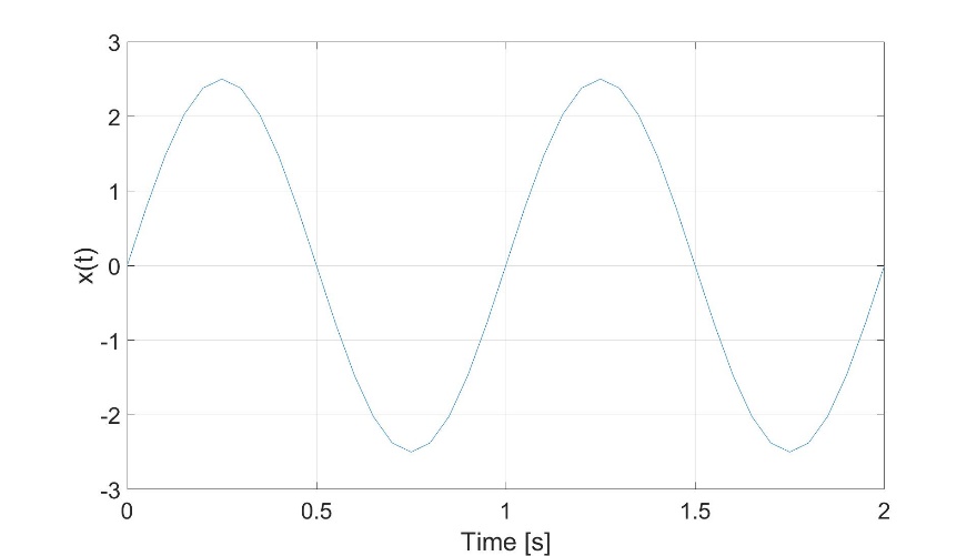
Fig. 474 Signal 1 in time domain, 2s (41 samples)

The signal has a length of 2 seconds and is sampled with 20 Hz. Thus, the signal consists of 41 samples. Transforming the signal into the frequency domain leads to the following spectrum:
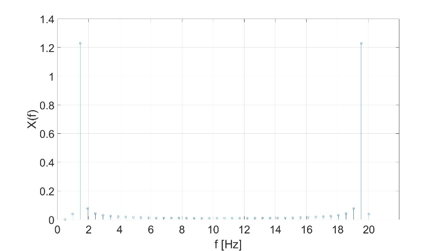
Fig. 475 Signal 1 in frequency domain, no zero-padding
The spectrum consists of 41 bins and the peaks @1 Hz and 19 Hz are clearly visible.
Now, the signal length is enhanced from 41 samples to 64 samples by adding 23 samples at the end of the signal:
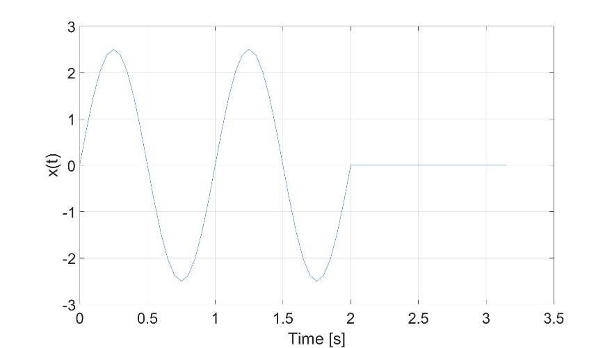
Fig. 476 Signal 1 in time domain, zero-padding to 64 samples
Transforming the signal to the frequency domain leads to the following spectrum:
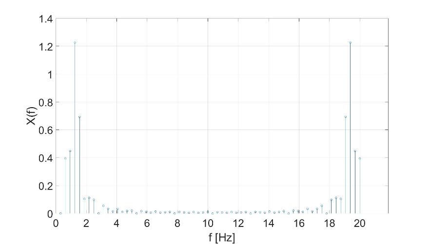
Fig. 477 Signal 1 in frequency domain, zero-padding to 64 samples
Now the spectrum consists of 64 samples and not 41 samples and the additional frequency bins are kind of an interpolation but do not lead to a sharper spectrum.
The same trend is visible if the original signal is enhanced from 41 samples to 128 samples by adding 87 zeros at the end of the signal:
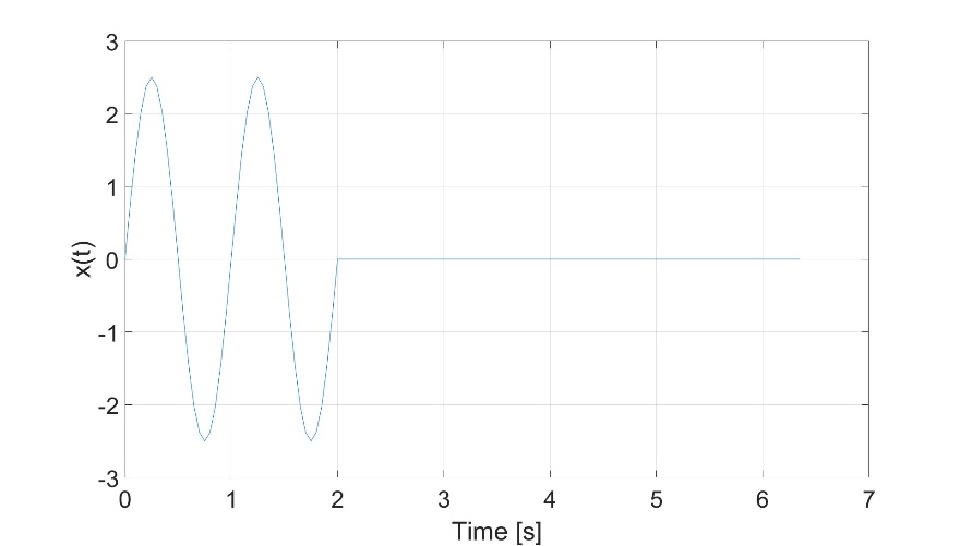
Fig. 478 Signal 1 in time domain, zero-padding to 128 samples
This signal leads to the following spectrum with 128 frequency bins:
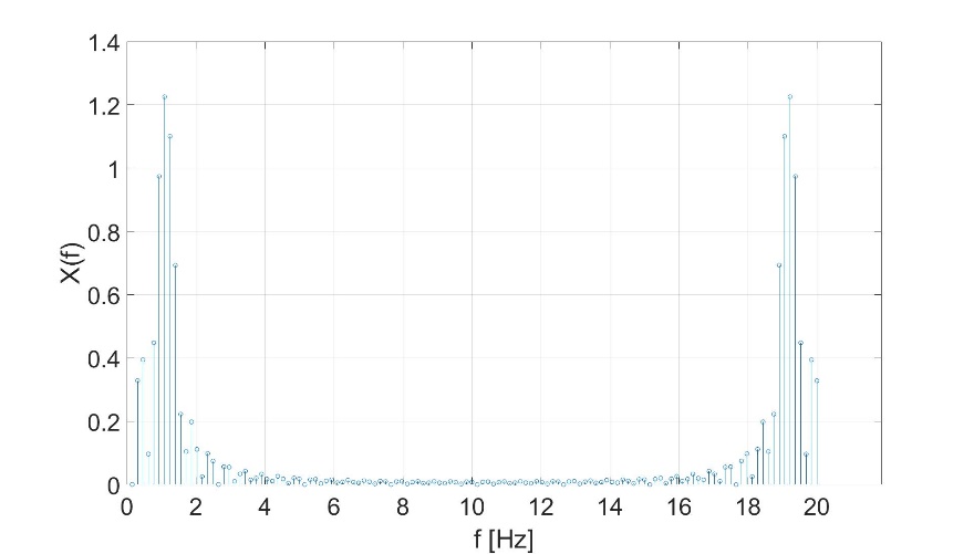
Fig. 479 Signal 1 in frequency domain, zero-padding to 128 samples
Again, the additional bins are only kind of an interpolation, but do not lead to a sharper spectrum.
To enlarge the accuracy of the FFT, a longer signal in time domain is required. Therefore, the original sine signal is enlarged to 6.4 seconds (128 samples):
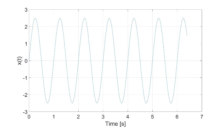
Fig. 480 Signal 2 in time domain, 6.4s (128 samples)
The resulting spectrum consists also of 128 bins but now, the additional bins really lead to a sharper spectrum and are no longer only an interpolation of the original 41 frequency bins:
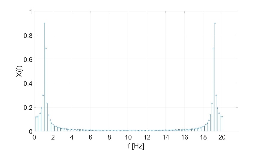
Fig. 481 Signal 2 in frequency domain, no zero-padding
Normalization of FFT Spectra
In this section, the necessity of the normalization during the FFT calculations is explained. Therefore a 50 Hz sine wave with 2.5 amplitude shall be transformed to the frequency domain. The sample rate is 1000 Hz and the signal length 10s. The signal looks as follows in time domain:
Fig. 482 Signal in time domain (first 250 ms)

After transforming the signal into the frequency domain according to the formula
and determining the absolute value, the spectrum is the following:
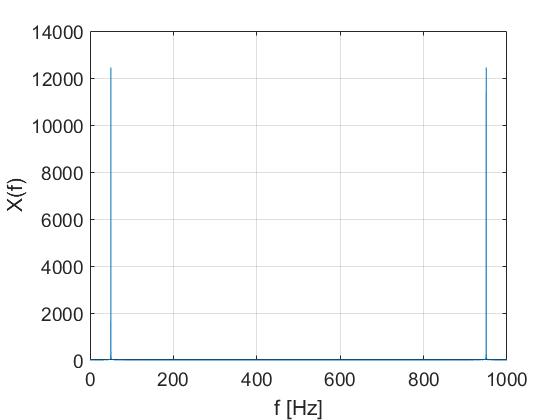
Fig. 483 x(t) in frequency domain
Two things are peculiar:
As the FFT produces a two-sided spectrum, there is a bin @ 50 Hz and @ 950 Hz.
As the signal level of the two peaks is ~12500, the unit seems to be arbitrary.
To create a comprehensible signal unit, the Fourier Transform of the signal must be divided by the length of the FFT which is 10001 in this example.

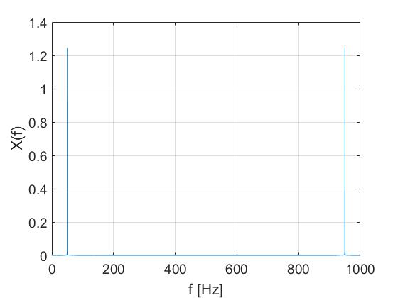
Fig. 484 x(t) in frequency domain divided by the FFT-length
Now, the amplitude of both peaks is ~1.25. As we still have two peaks whose sum is ~2.5, the signal unit issue is solved by dividing the spectrum by the length of the FFT.
In a next step, we truncate the spectrum at the Nyquist frequency ( ) which is 500 Hz in our case and multiply the remaining spectrum from 0 to 500 Hz with the factor 2 to ensure that the power of the signal in the frequency domain is still the same as in the time domain. After that, the following spectrum results:
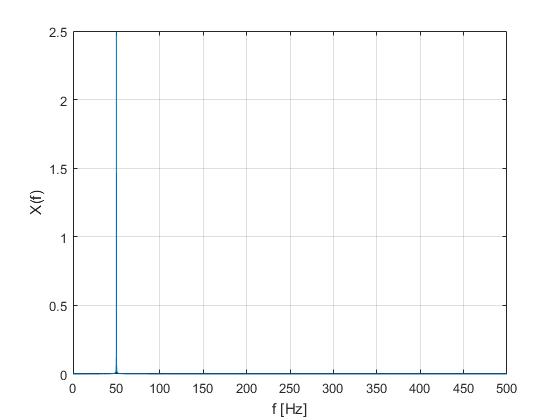
Fig. 485 One-sided spectrum X(f) multiplied by factor 2
In this first example, there is no normalization needed, because we didn’t use a window function. In this case, there was no window function needed, because we transformed a finite and periodical signal. In practice, this is normally not the case and a continuing signal is transformed block by block. As these block lengths are finite, the Leakage effect occurs if the block length does not coincidentally match with an integer multiple of the signal period. In this case, the frequency spectrum becomes too wide. This is a natural effect resulting from the Fourier Transform property which says that a multiplication in time domain leads to a convolution in the frequency domain. The fact that the frequency spectrum becomes too wide can be optimized but not completely rejected by the usage of a window function. This leads to the fact that the signal is faded in at the beginning of the window and faded out at the end of the window. Thus, an artificial periodical signal results and an error in the signal amplitude results. This amplitude error is corrected by the normalization of the signal.
Let’s assume again the 50 Hz sine wave with 2.5 amplitude shown in Fig. 482 and multiply it with a Hanning window. The formula for the creation of a Hanning window can be found in section Window type. After the multiplication, the signal looks as follows:
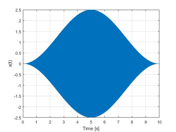
Fig. 486 x(t)win in time domain; multiplied with a Hanning window

The spectrum of the signal looks as follows:
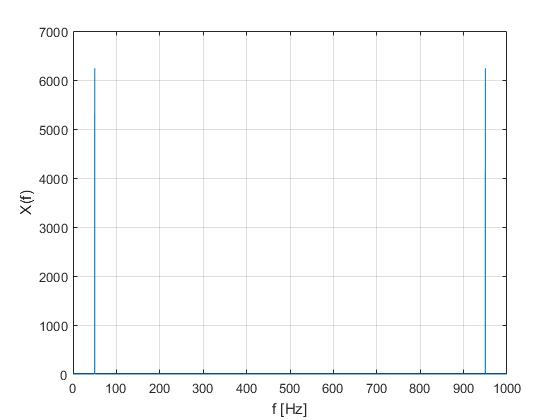
Fig. 487 x(t)win in frequency domain
Again, the signal unit looks arbitrary. Thus, we divide the spectrum by the length of the FFT (N=10001) again.

Fig. 488 x(t)win in frequency domain divided by the FFT-length
After that we truncate the signal again at the Nyquist frequency and multiply the remaining spectrum with the factor 2 to secure that the signal power in time and frequency domain is equal.
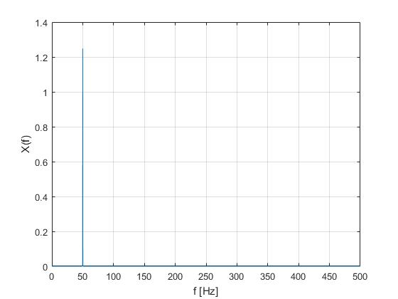
Fig. 489 One-sided spectrum X(f)win multiplied by factor 2
Now we clearly see that the peak @50 Hz is not 2.5 as before but only ~1.25. This is because of the windowing. This can be corrected with the normalization. There are two possibilities: We can either normalize the spectrum to the original signal amplitude or to the original signal power.
To refit the spectrum according to the original signal amplitude, we must select the Amplitude True normalization:
where N denotes again the window (and signal) length and Wk the value of the window function at position k.
There we can see that the peak @50 Hz is again 2.5. But in this case, the signal power in frequency domain is not the same as in time domain. If this is required, we must select the Power True normalization:
where N denotes again the window (and signal) length and Wk the value of the window function at position k.
Now, the power in frequency domain is the same as in time domain, but the amplitude does not match correctly anymore.
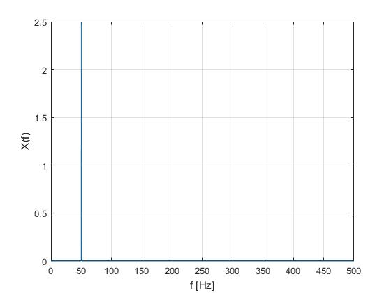
Fig. 490 Amplitude-True-normalized spectrum X(f)

Fig. 491 Power-True-normalized spectrum X(f)
Calculation of the Periodogram - Averaging of FFT windows
This section will demonstrate the calculation of a periodogram in a practical example. The exemplary window size is 1000 samples. The following figures illustrate the decomposition of a time signal for the calculation of a periodogram:
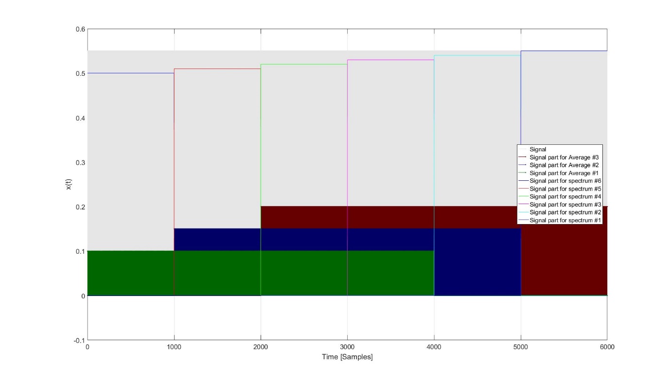
Fig. 492 Decomposition of the time signal for a Periodogram with an average of 4 spectra and 0 % overlapping
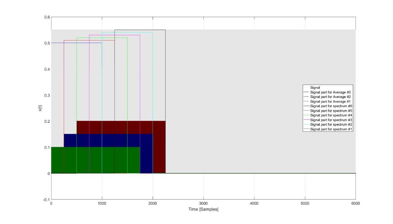
Fig. 493 Decomposition of the time signal for a Periodogram with an average of 4 spectra and 75 % overlapping
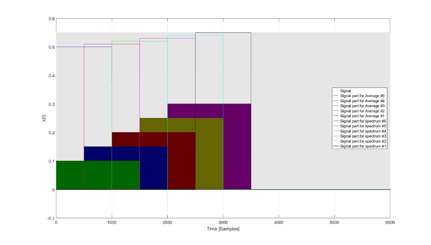
Fig. 494 Decomposition of the time signal for a Periodogram with an average of 2 spectra and 50 % overlapping
Auxiliary
Image instrument
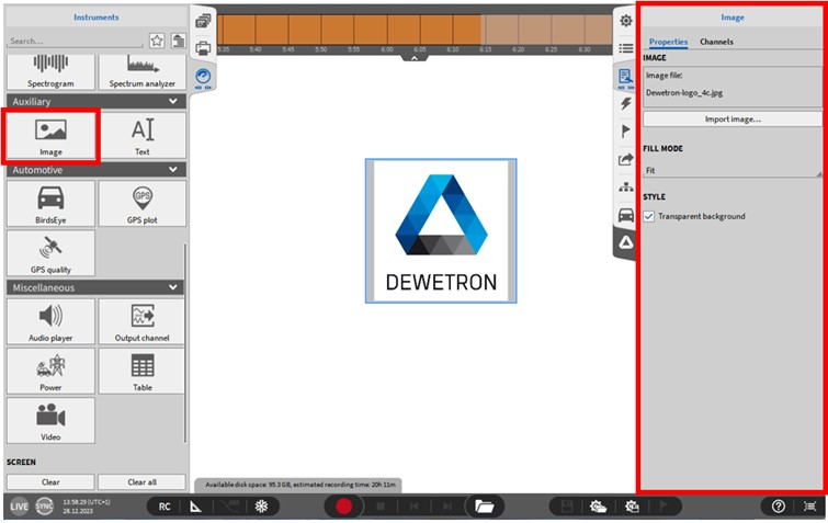
Fig. 495 Image Instrument – overview
This feature allows the user to add an image to the measurement screen, i.e. a picture of the device under test or the company logo. The data path can be selected via the Instrument Properties:
Source: Browse for the desired image file
Fill Mode: Select different modes to adjust the image file to the Instrument size
Style: Selection of a transparent or untransparent background.
Layer: Moves the Instrument in front of or behind another object (only applicable in Design Mode).
Note
An image file (.jpeg or .png) can also be copied and pasted directly from the Windows Explorer into the OXYGEN measurement screen (see Fig. 496).
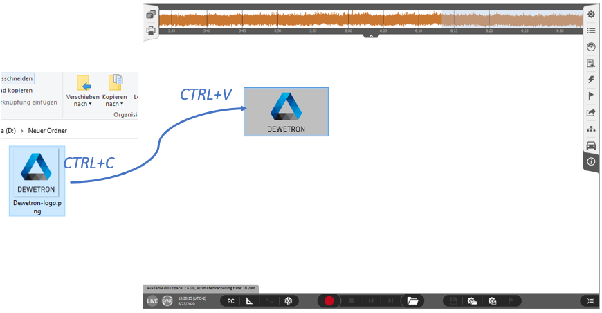
Fig. 496 Pasting an image file to the measurement screen
Text instrument
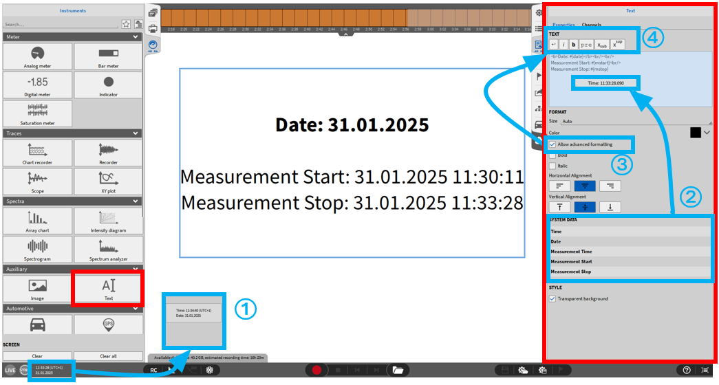
Fig. 497 Text instrument – overview
This feature allows the user to create customized text items on the measurement screen. Header data, time, data and the measurement time can also be displayed in the Text Box. For a detailed description how to display header data in the text box refer to Header data, for the other features see the next section. The following Instrument Properties are available:
Text: the desired text must be entered there. The entered text is automatically resized to fit within the boundaries of the text box. To change the color of the text, left click onto or touch the Color square to bring up the color selection palette. The style can be adjusted to Bold and Italic. Furthermore, the horizontal and vertical alignment can be changed. The advanced text formatting options (see ④ in Fig. 497) for formatting only certain words or characters instead of the entire text must be activated via the checkbox (see ③ in Fig. 497).
Style: Selection of a transparent or untransparent background.
Layer: Moves the Instrument in front of or behind another object (only applicable in Design Mode).
Note
A text can also be copied and pasted directly to the OXYGEN measurement screen (see Fig. 498).
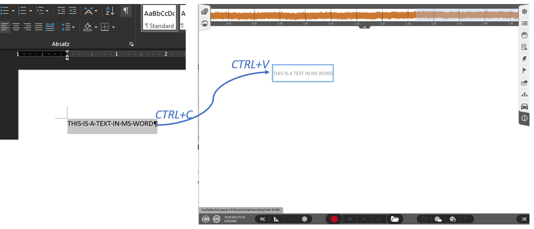
Fig. 498 Pasting a text to the measurement screen
Show Time, Date, Measurement Time
The Text instrument can also be used to show time, date or the elapsed time since measurement start (recording start) on the measurement screen. It is also possible to select the start and end time of the measurement. There are two possibilities available:
The time and date display in the lower left corner can directly be dragged and dropped on the measurement screen (see ① in Fig. 497). A Textbox will be created automatically with the according time and date.
In the instrument properties the time, date and measurement time can again dragged and dropped into the text field (see ② in Fig. 497) or be added with a double click on the respective element.
Note
The text in front of the #-sign can be changed individually.
Automotive
GPS plot
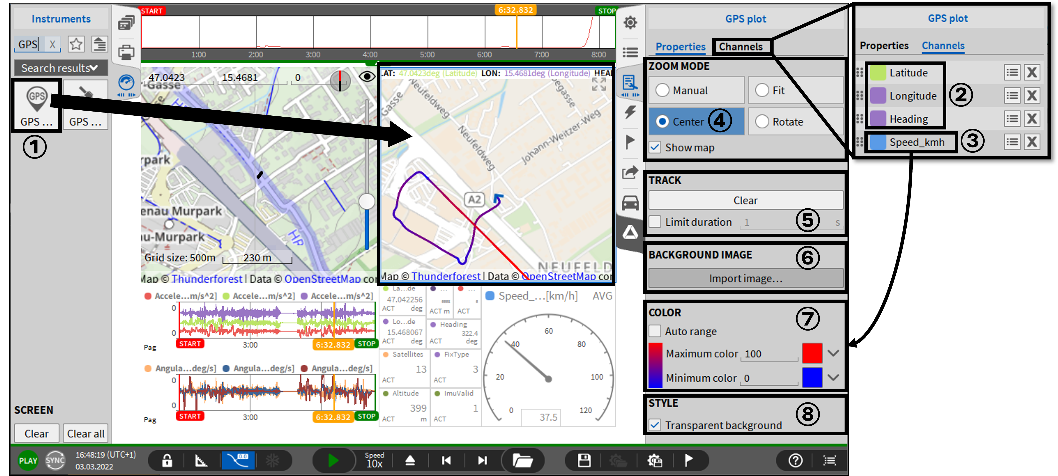
Fig. 499 GPS plot instrument - overview
The GPS plot instrument ① displays Latitude, Longitude, and Heading channels acquired by TRION-TIMING or TRION-VGPS modules (see GPS channels). These channels are automatically assigned the LAT, LON, and HEAD based on their channel mode ②.
Alternatively, mathematical channels (e.g., Statistics channels) can be assigned to the GPS plot, but they must be assigned in a specific order (Latitude, Longitude, Heading) and cannot be automatically matched. A fourth channel, such as speed, can be added to create a color trail based on a defined minimum and maximum value and color ③.
The displayed map is an online OpenStreetMap, which can be stored in the cache for offline viewing.
The user can manipulate the following Instrument Properties:
④ ZOOM MODE
Manual: The user can zoom with the scroll wheel and move the map with the left mouse button. The actual position will not be centered when the position is updated.
Fit: The complete track of the object is visible in the Instrument. Zooming or moving is not applicable.
Center: The actual position of the tracked object is always displayed in the center of the Instrument. Zooming with the scroll wheel and moving with the left mouse button is possible but the actual position will be centered again when the position is updated.
Rotate: The actual position of the tracked object is always displayed in the center of the instrument and the heading shows always to the top. Zooming with the scroll wheel and moving with the left mouse button is possible but the actual position will be centered again when the position is updated.
Show Map: Toogle if the Open Street map is shown or not.
⑤ TRACK
The elapsed track will be deleted by clicking on the Clear button. The drawing of the elapsed track can be limited by entering a time in seconds in at Limit duration
By default the whole track is displayed as no limit is active.
⑥ BACKGROUND IMAGE
For offline usage, an image can be loaded to replace the map. An image can be selected by clicking on the Import Image button and browsing for the desired file. After selecting the desired file, the Positioning dialog will open:
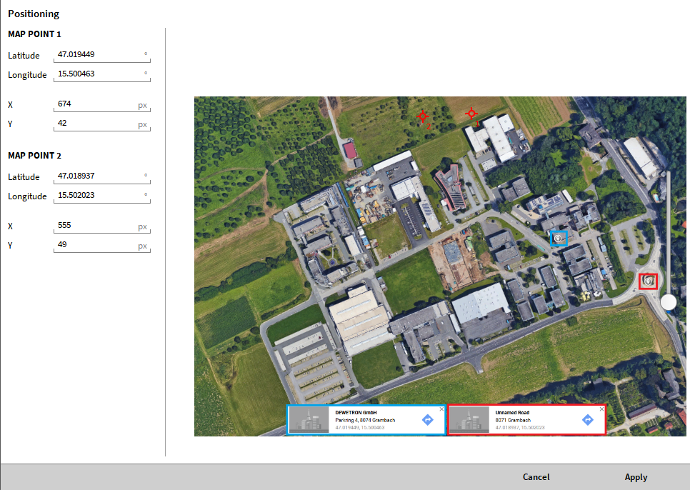
Fig. 500 Image positioning dialog
Two GPS coordinates within the loaded image must be known to position the image correctly. In Fig. 500, the two points and their corresponding coordinates are marked with red and blue. The procedure to position the image is the following:
Two red cursors are generated by the Positioning dialog. In Fig. 500, they can be found at the top of the image. These cursors must be put on the known coordinates.
The coordinates of both known points must be entered.
Latitude and Longitude of MAP POINT 1 must be entered for the known coordinates the first red cursor is placed on. In Fig. 500, this is the GPS coordinate marked with blue
Latitude and Longitude of MAP POINT 2 must be entered for the known coordinates the second red cursor is placed on. In Fig. 500, this is the GPS coordinate marked with red
Alternatively, the image pixel corresponding to MAP POINT 1 and MAP POINT 2 can be entered in the X and Y columns
After the positioning is finished and clicking on Apply, the image is placed correctly on the map (see Fig. 501):
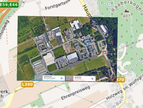
Fig. 501 Positioned image
⑦ COLOR
Auto range accounts for the channel range as maximum and minimum of the color trail. The default color between the maximum and minimum is deactivated per default and can be activated additionally with the respective checkbox.
The color of maximum, minimum and default color as well as the values can be freely chosen
⑧ STYLE
Transparent background: Toggles background opacity.
GPS quality
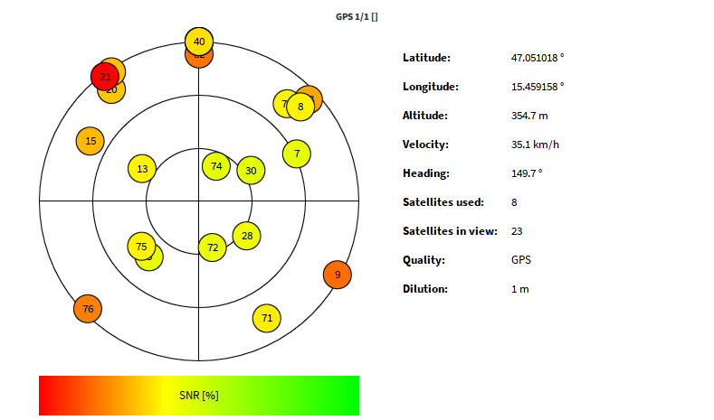
Fig. 502 GPS Quality instrument - overview
The GPS quality instrument displays the number of visible and used satellites of GPS data which is acquired by a TRION-TIMING or TRION-VGPS-20/-100 module (see GPS channels) and further meta data. The used satellites are thereby the satellites with the best SNR. The NMEA data channel can be assigned to the GPS quality instrument. Normally, the NMEA data channel is called GPS 1/1 per default and can be found on the top of the GPS data channels list:
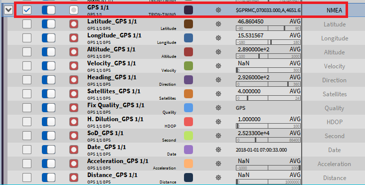
Fig. 503 GPS NMEA data channel
Besides the satellites plot, the following meta data which is contained in the NMEA string can be displayed in the GPS quality instrument:
Latitude
Longitude
Altitude
Velocity
Heading
Satellite used
Satellites in view
Quality
Dilution
The following Fig. 504 explains the meaning of the three black circles with the same center point in the satellites plot:
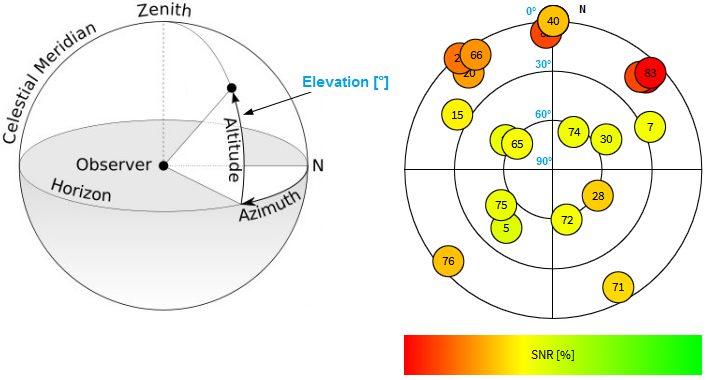
Fig. 504 Explanation of the satellites plot
The deselection of the instrument property Extended View reduces the content of the GPS plot Instrument to the satellites plot:
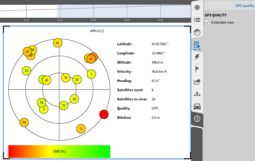
Fig. 505 GPS quality instrument - Extended View selected
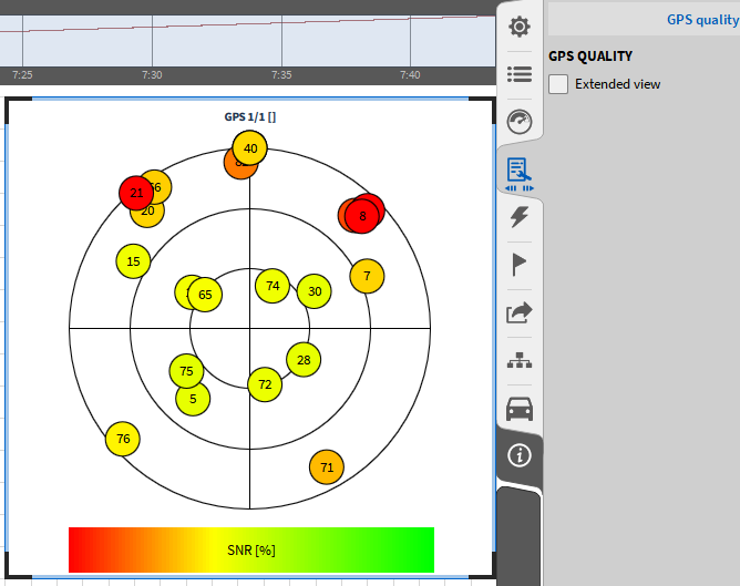
Fig. 506 GPS quality instrument - Extended View deselected
Miscellaneous
Polar plot
The polar plot complements the orbit analysis and is also a pure display instrument without its own channel. The Polar Plot can be used to display a vector signal in polar coordinates, for example the amplitude and phase of the X deflection for the 1st order in relation to the speed of a shaft. In the polar plot, the amplitude is displayed as a radius and the phase as an angle. The amplitude and phase are calculated using order analysis.
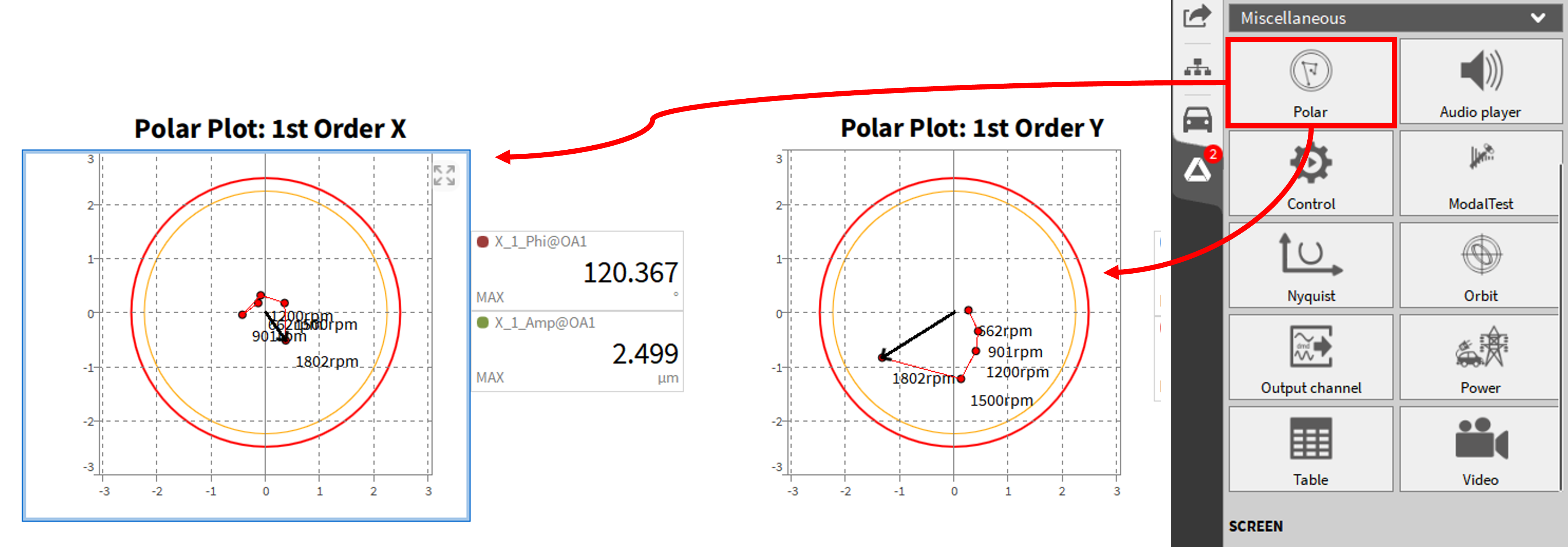
Fig. 507 Polar Plot Instrument Overview
Example of Polar Plot settings
Only rotational speed, amplitude and phase from order analysis (requires OXY-OPT-OA) are required for the polar plot. As in the orbit plot, the display is scaled via the free space/bearing clearance diameter ① with a red circle and a limit ② based on this. The steps in which the movement vector is marked by a point can be defined by speed or time ③ in the input field ④. The length of the polar vector represents the amplitude, and the angle represents the phase offset to the starting point of the encoder revolution. This means that for the following example at 2700 rpm, the maximum X-deflection is ~13 µm and is ~145° offset from the speed signal.
Note
The Order analysis calculates the amplitude based on the RMS values, and for Peak or Peak-Peak scaling, the scaling must be done in the channel list.
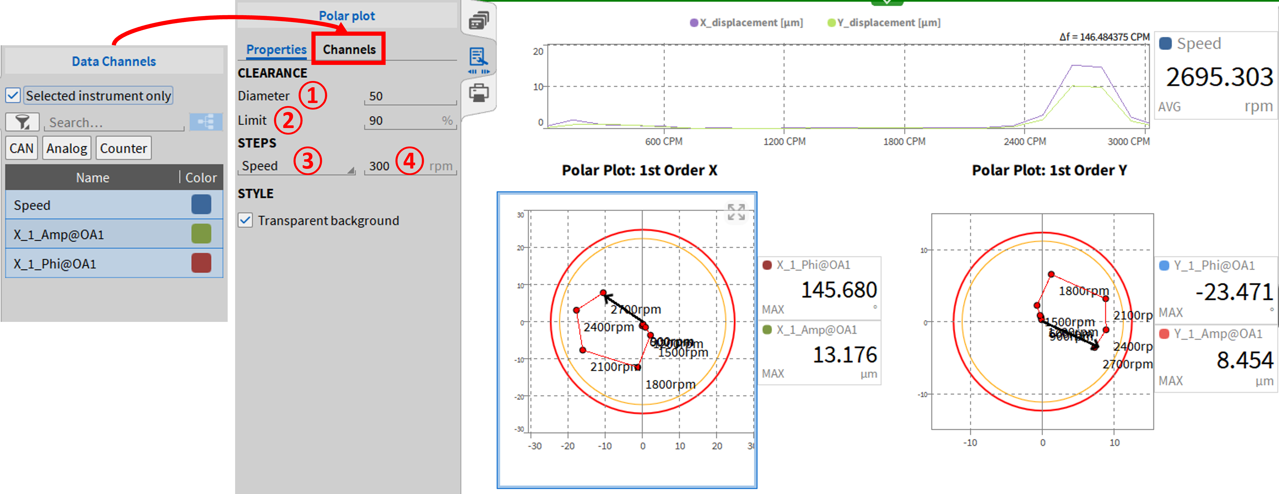
Fig. 508 Polar Plot properties and assigned channels
Audio Player
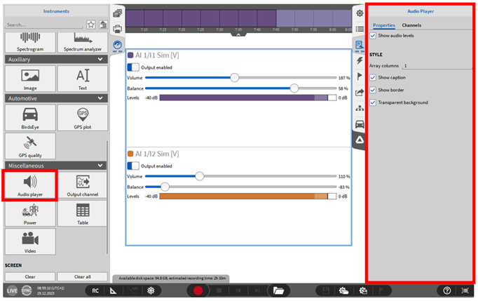
Fig. 509 Audio Player instrument - overview
The Audio player Instrument can be used to replay OXYGEN channels via the systems’ default sound card.
The instrument provides the possibility to mute the channel(s) (Output enabled), to set the output Volume and to change to left-right Balance (see Fig. 509).
The maximum number of channels to be assigned to one Audio Player is 2. It is possible to replay synchronous data channels (i.e. analog inputs and formulas).
The recommended channel sample rate is from 1 kHz to 200 kHz.
Style: Selection of a transparent or untransparent background.
Show short channel name. This option does not display the node or group channel name in case the channel name has one. “AI 1/1@DEWE3-RM16” will be displayed as “AI 1/1” with the activated option.
The audio replay functionality is available in LIVE, REC and PLAY mode. In LIVE and REC mode, the actual data is replayed. In PLAY mode the replay is snapped to the position of the Orange cursor (see Fig. 510).
Fig. 510 Orange cursor in Overview bar and Recorder
Control instrument
The Control instrument is available under the Miscellaneous category in the Instrument tab. Its functionality depends on the selected control type. The available control types are:
Shunt: Turn all shunts on or off for all analog channels in bridge mode.
Note
This action can also be used during recording.
Bridge balance: Perform bridge balancing for all active analog channels in bridge mode.
Saturation data: Reset saturation data for all channels.
Control type: Shunt
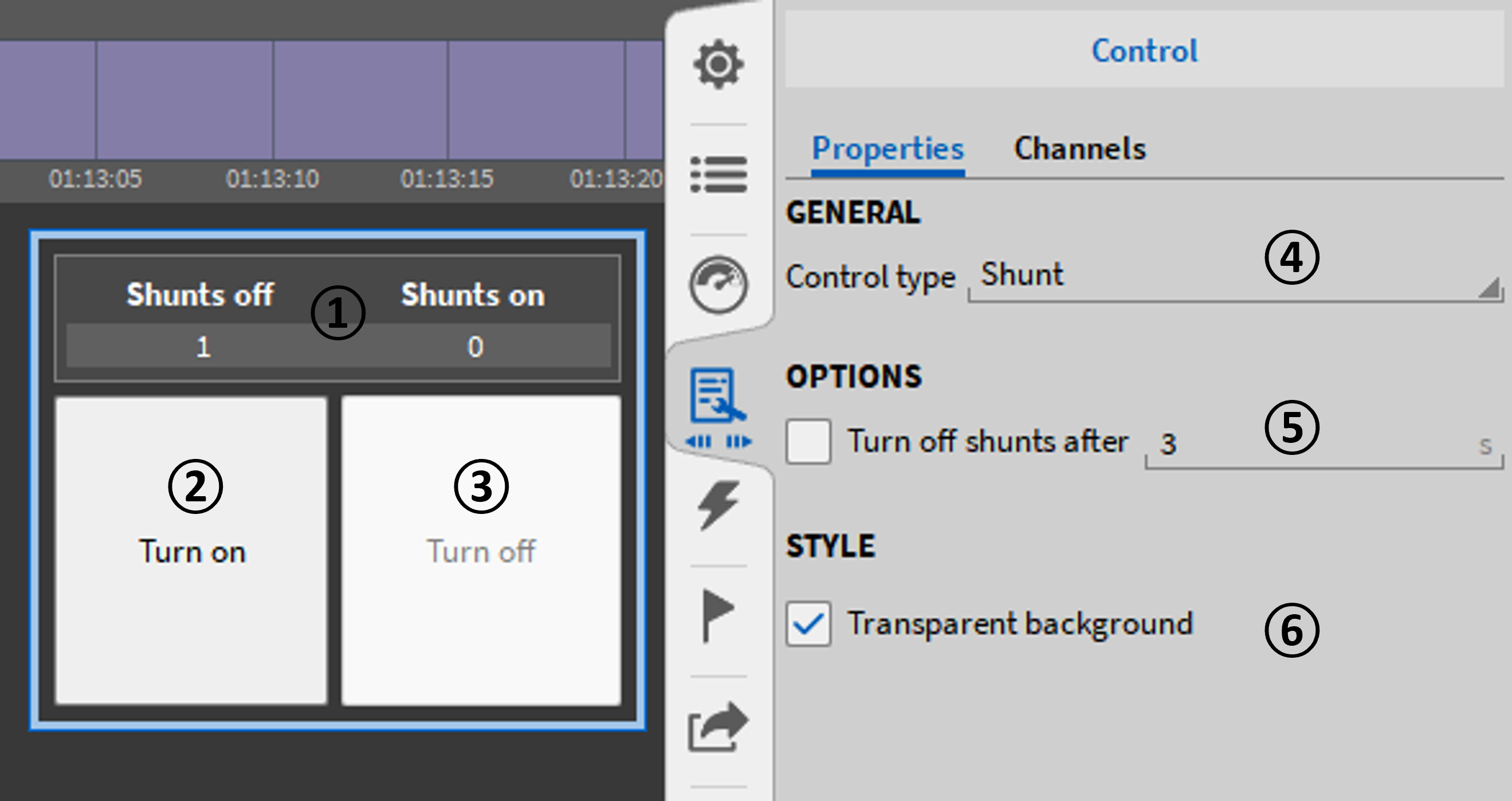
Fig. 511 Control instrument properties for control type: shunt
No. |
Function |
Description |
|---|---|---|
1 |
Caption |
Control type title; shows the number of deactivated and activated shunts for all channels in bridge mode. |
2 |
Control action |
Action button to turn on/off all shunts for all channels in bridge mode; can be used during recording. |
3 |
General properties |
Select the desired control type |
4 |
Control type-specific options |
Checkbox to automatically turn off shunts after a specified duration (1 to 60 seconds). |
5 |
Instrument style properties |
Tick box to: - Enable/disable a transparent background. - Show/hide caption. |
Control type: Bridge balance
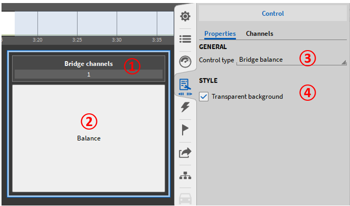
Fig. 512 Control instrument properties for control type: Bridge balance
No. |
Function |
Description |
|---|---|---|
1 |
Caption |
Control type title; shows the number of channels in bridge mode. |
2 |
Control action |
Action button to perform a bridge balance for all channels in bridge mode. |
3 |
General properties |
Select the desired control type. |
4 |
Instrument style properties |
Tick box to: - Enable/disable a transparent background. - Show/hide caption. |
Control type: Saturation data
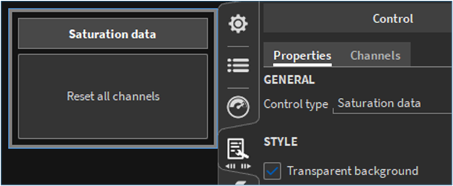
Fig. 513 Control instrument properties for control type: Saturation data
No. |
Function |
Description |
|---|---|---|
1 |
Caption |
Control type title |
2 |
Control action |
Action button to reset saturation information for all channels. |
3 |
General properties |
Select the desired control type. |
4 |
Instrument style properties |
Tick box to: - Enable/disable a transparent background. - Show/hide caption. |
Nyquist Plot (SDOF circle fit)
The Nyquist plot is an instrument that can numerically determine the natural frequency, and the loss factor based on the frequency response function (FRF) channels from the Modal Test. The data is plotted in a circle and interpolated. There is also a corresponding screen template for this instrument.
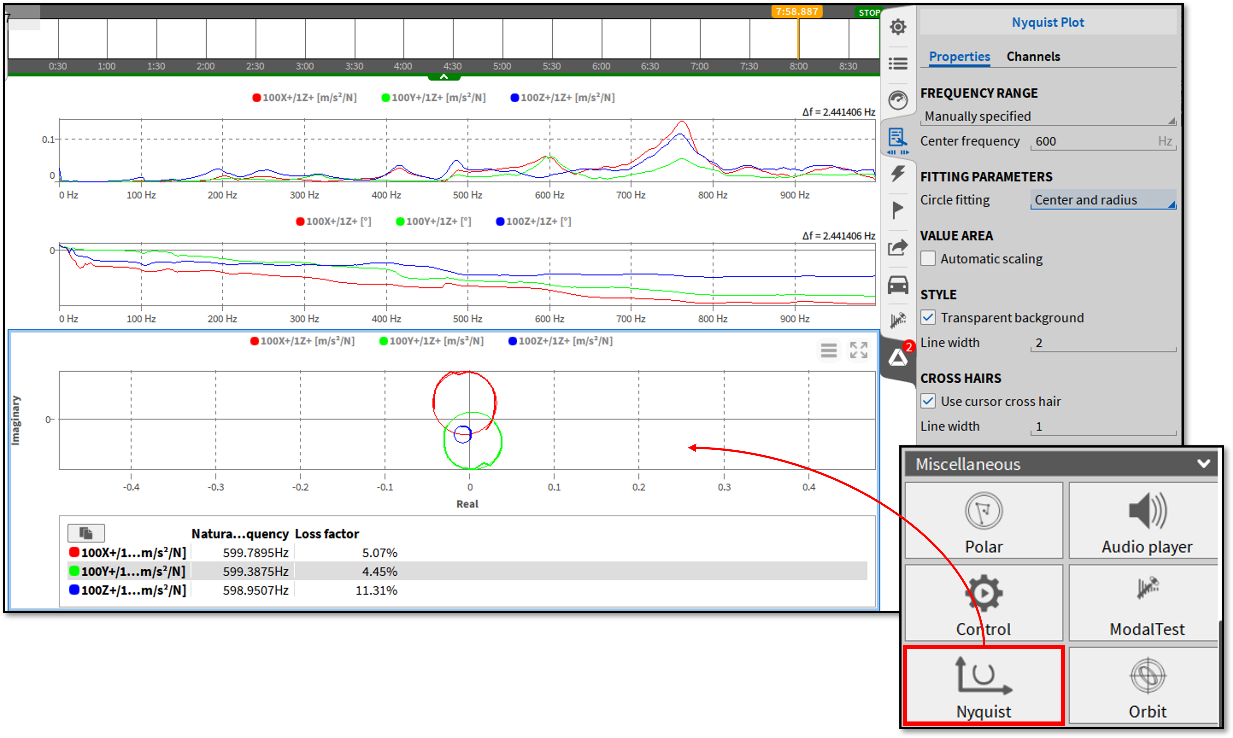
Fig. 514 Nyquist Plot properties
Further information on the modal test and the Nyquist plot can be found in the Modal Test manual: DEWETRON_Oxygen_Modal_Technical_Reference_vx.x (https://ccc.dewetron.com/).
Orbit plot
The orbit plot is an instrument for displaying the rotational axis movement for e.g. turbine shafts. A minimum of 2 signals for the deflection of the shaft are always required. The angle between the X and Y signals on the test object is always assumed to be 90°.
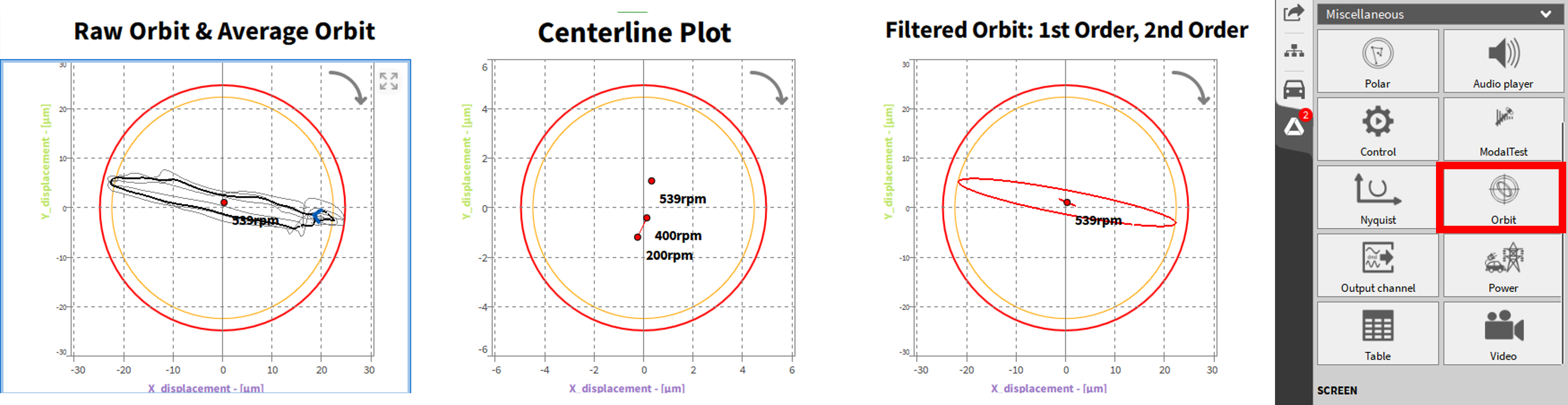
Fig. 515 Orbit plot Instrument
The Orbit plot has three display options, which can be activated individually or in combination in the instrument settings, but some of them require different input signals. The scaling of the input channels must be carried out in advance in the channel list. The Orbit plot is a pure display instrument, i.e. there are no separate Orbit plot channels.
For the display options the following Input channels are required:
Raw orbit & average orbit: X&Y deflection + optional angle and speed
Centerline plot: X&Y deflection + angle + speed
Filtered orbit: X&Y deflection + amplitude and phase in X and Y direction per order + angle + speed
For this view the order analysis license option (OXY-OPT-OA) is required.
The next figure shows an example for X- and Y-Probe arrangement. Additionally, the context of the orbit in a bearing is illustrated. The start and orbit direction are also displayed in OXYGEN.
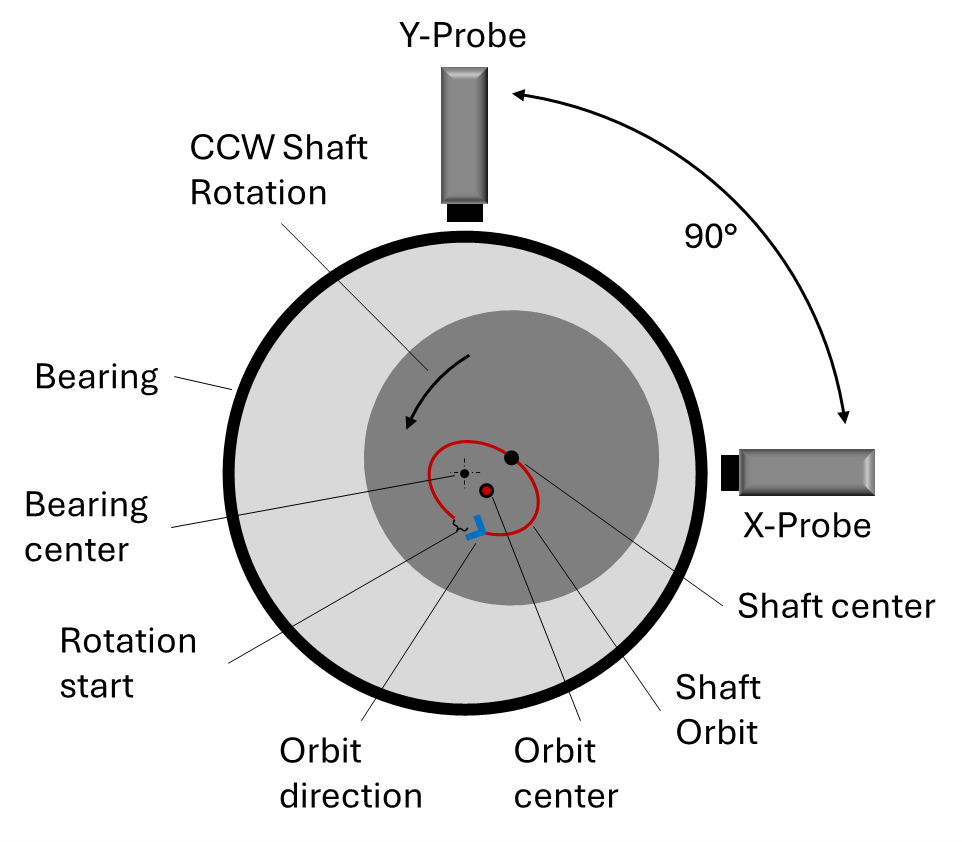
Fig. 516 X&Y Probe arrangement and Orbit overview
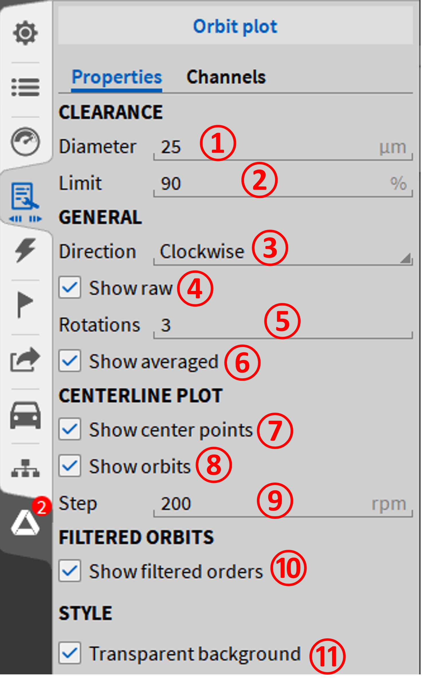
Fig. 517 Orbit plot Instrument properties
The settings ①, ② and ③ are relevant for all orbit plot types, as the diameter ① is used to set the rotation in relation to a circular clearance/bearing. In this view, the limit ② helps to easily recognize when a movement radius is exceeded. The direction of rotation of the test can simply be marked via ③ but has no further effect on the display or calculation in the background. The other settings are explained in the following examples.
No. |
Property |
Description |
|---|---|---|
① |
Diameter |
Determines the display scale in the form of a red circle, representative of a clearance/bearing play. |
② |
Limit |
Limit display in % in relation to the clearance/bearing play diameter. |
③ |
Direction |
For reporting purposes, the direction of rotation of the shaft is displayed in the instrument (clockwise/counter-clockwise) |
④ |
Show raw |
Shows the unaveraged orbit of the rotation axis over x revolutions |
⑤ |
Rotations |
Defines the number of orbits displayed in ④ and ⑥. |
⑥ |
Show averaged |
Displays the average orbit over x revolutions. The revolutions for the center position are defined in ⑤. |
⑦ |
Show center points |
Shows the calculated center of the orbits in x speed steps, which is defined in ⑨. |
⑧ |
Show orbits |
Also shows the center of the orbits between the defined speed steps. |
⑨ |
Step |
Defines the speed increment for the center points ⑦. |
⑩ |
Show filtered orders |
Displays the filtered orbit |
⑪ |
Transparent background |
Sets the instrument background to transparent |
Example of Raw orbit and Average orbit
X and Y deflection in length dimension are required for the raw and average orbit. If no angle and speed signal is assigned, OXYGEN plots one sample per degree and can therefore still estimate an average over x revolutions. In Fig. 518 three orbits are displayed in grey and their average is shown with a black and bold line.
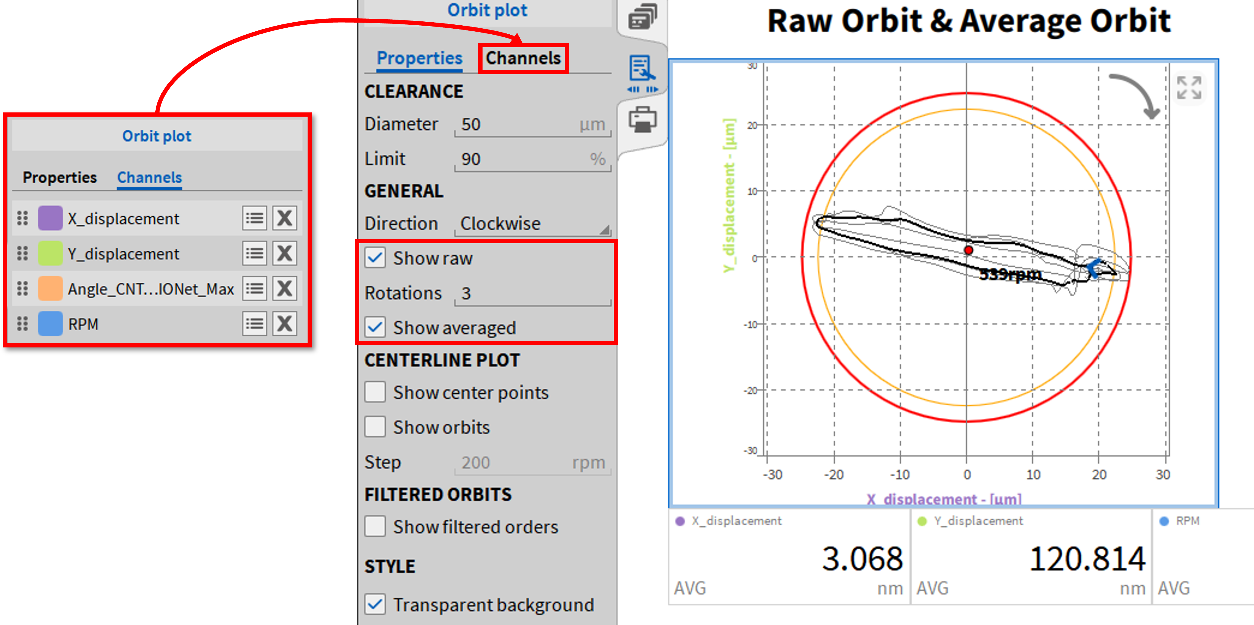
Fig. 518 Raw Orbit and Average Orbit
Example of Centerline Plot
In addition to X and Y deflection, angle and speed are always required for the centerline plot. The center points are saved as a snapshot after a short dwell time close to the step size. The calculated center points can be displayed before the snapshot using Show orbits.
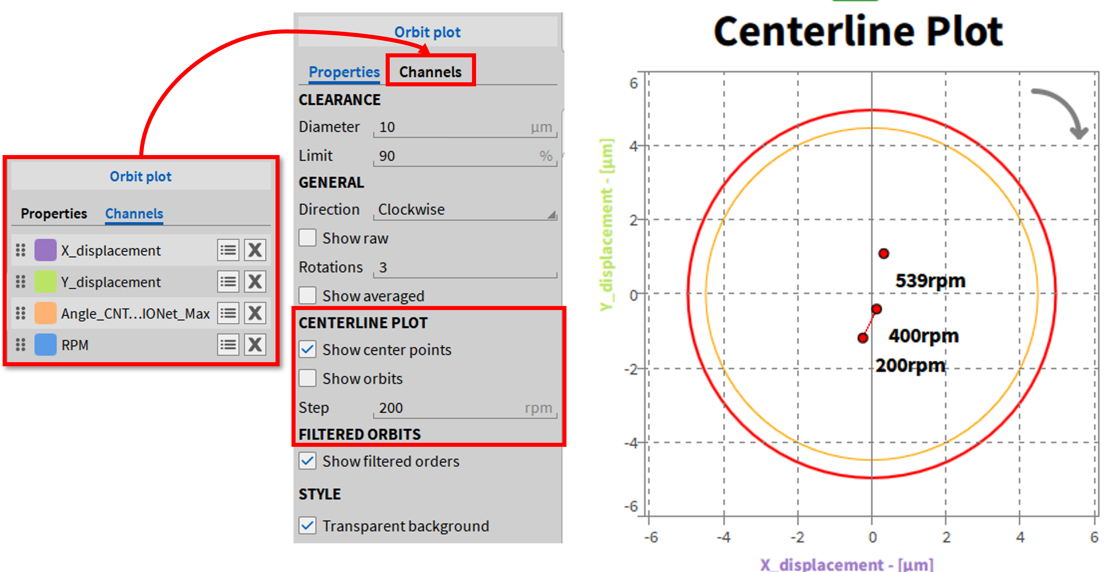
Fig. 519 Centerline Plot Example
Example of Filtered Orbit
Based on the amplitude and phase channels of the order analysis (from order analysis), filtered orbits can be used to display the orbit with the same or multiple fundamental frequency in relation to the speed. Speed and angle as well as X and Y deflection channels are required. Amplitude and phase must be assigned for X and Y for each order.
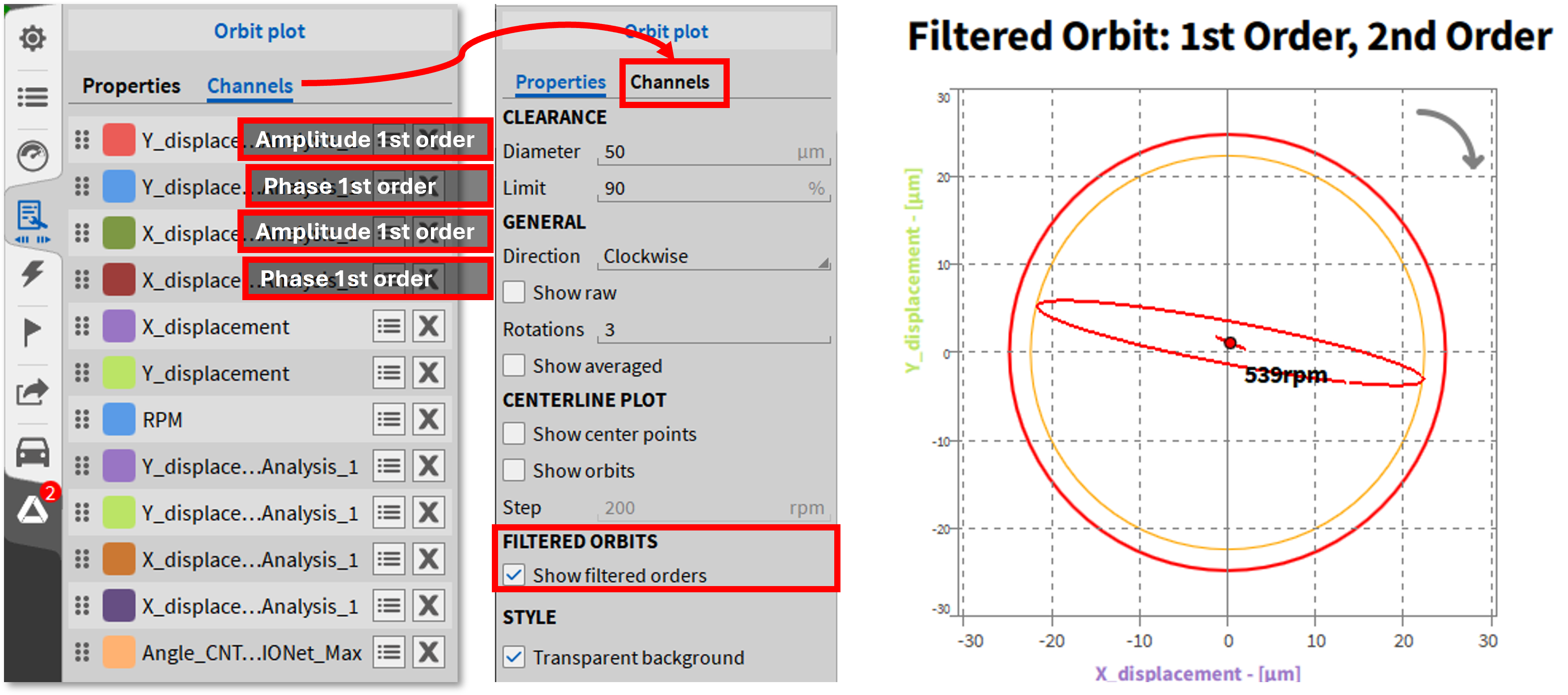
Fig. 520 Filtered Orbit Example for 1st and 2nd Ordnung based on Order analysis
Output Channel
Fig. 521 Output Channel instrument
The Output Channel Instrument can be used to set the AOUT channels (Analog Output Channels) in the measurement screen. Channels that are set as constant value output or function generator can be displayed and changed here.
Up to 8 channels can be assigned to an Output Channel Instrument. The functions of the Output Channel Instrument are available in LIVE and REC mode.
Power Group
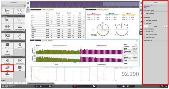
Fig. 522 Power Group instrument – overview
OXYGEN Power is the up to date Power Analyzer software add-on for DEWETRON OXYGEN Measurement Software. For a detailed explanation of the functionality and usage of the Power module, refer to the manual DEWETRON_OXYGEN_Power_Technical_Reference_Rx.x.
Table instrument
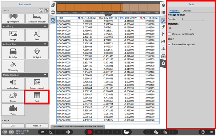
Fig. 523 Table instrument - overview
The Table instrument displays measurement data in tabular format, with individual columns for each signal and one for the time axis. Per Default the newest values will be listed at the top of the table instrument and the oldest ones at the end, with the setting “Reverse Time” this order can be switched. When the measurement is freezed or if the table will be used in a previously recorded measurement file it is possible inside the instrument to scroll between the values with the scroll wheel of the mouse. The following configuration options are available:
Time Format: Choose between Auto, Absolute time, or Relative time.
Number Precision: Set the number of decimal places displayed.
Reverse time: The order of the values can be switched. If deactivated the newest values will be listed at the top of the instrument, if activated, the newest values will be listed at the end.
Column Layout: Select from Equal width, Dynamic distribution, or Stable distribution.
Statistics Display: Enable Show only statistics data to display statistical values instead of raw data. Use the dropdown menu to select specific statistics. Note: Statistics Recording (Triggered Events) must be enabled during acquisition for this feature to work.
Style: Choose between a transparent or non-transparent background.
Show short channel name: This option does not display the node or group channel name in case the channel name has one. “AI 1/1@DEWE3-RM16” will be displayed as “AI 1/1” with the activated option.
Note
Up to 8 channels can be assigned to one single Table instrument.
Video instrument
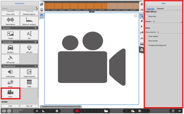
Fig. 524 Video instrument – overview
OXYGEN provides the possibility to record a video during the measurement. The following cameras types are supported:
USB webcams
DEWE-CAM-GIGE-120 and DEWE-CAM-GIGE-50-HD
ALVIUM 1800 U-240 and ALVIUM 1800 U-040
ALVIUM G1 and G5
For example, this is a very useful tool for automotive applications when a test run is performed, and the test track shall be recorded. Please note that the camera channels are not activated by default in a new setup. This can be changed in the Data Channels menu in the Video Channels section by clicking on the Activate switch. This will activate your plugged camera. For enabling the record mode as well, make sure that the Stored button has the red colored background (see Fig. 525).
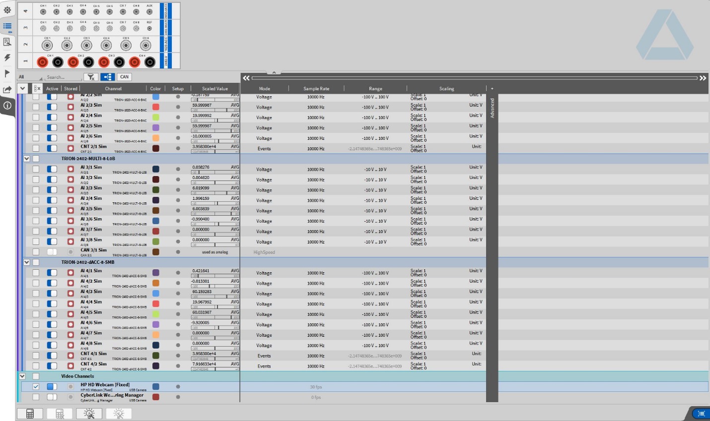
Fig. 525 Activate cameras and enable recording
After that the user can find the cameras in the Data Channel List of the Video Instrument and assign a video channel.
Note
The video recording with a webcam or a DEWE-CAM-GigE-120/-50-HD in fixed frame rate mode are not synchronized to the other measurement channels. When synchronized recording is required, OXYGEN supports time synchronous recording with a DEWE-CAM-GigE-120/-50-HD.
For the driver installation and the required software settings refer to the Installation Guide of the DEWE-CAM-GigE in OXYGEN.
Note
If the camera channel does not appear in the Channel List although a camera is connected to the measurement system, make sure that CAMERA Series for webcams or the GIGECAMERA Series for GigE cameras are enabled in the DAQ Hardware setup (see Fig. 526) in the System Settings.
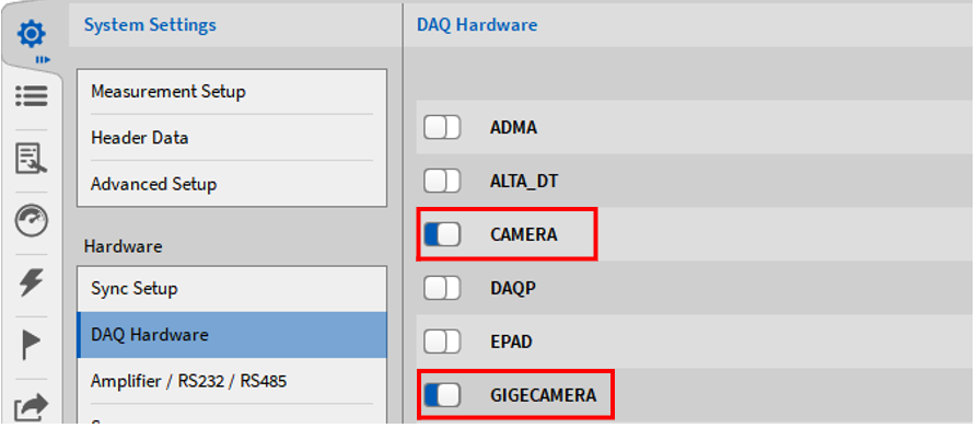
Fig. 526 Enabling the Camera Series and the GigE Camera series in the DAQ Hardware setup
The Video Instrument has the following Instrument Properties (see Fig. 524):
Video display
If Show time is selected, the current measurement time is displayed in the Video Instrument
Rotation of video picture by 90°, 180° or 270°
Style: The user can specify the number of columns if several channels are selected. Selection of a transparent or untransparent background.
Layer: Moves the instrument in front of or behind another object (only applicable in Design Mode).
Note
For each connected camera, there exists a counter channel that counts the number of received frames since acquisition start. The channel has the same name as the respective camera with RcvdCNT appended. To activate the counter, you need to activate the channel (The channel is not activated automatically). The channel can be found in the Video Channels section of the Channel List (see Fig. 527).
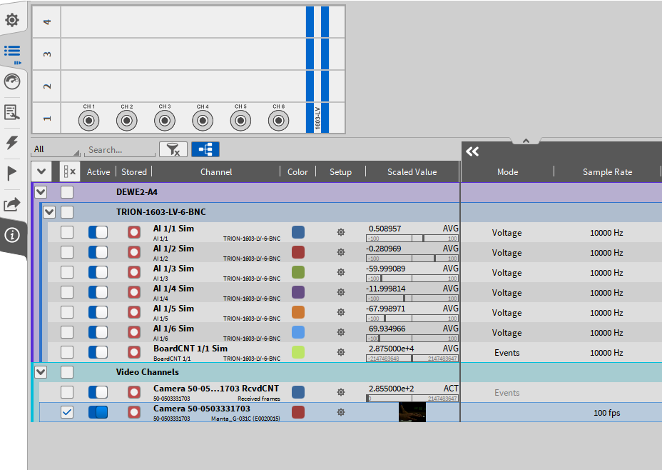
Fig. 527 Frame Counter Channel
Note
When using more than one USB camera, problems may occur under Windows 10® if they are connected on the same USB hub. The second camera (and others) may not work/show a picture. If more cameras shall be used, only one camera per USB hub should be connected to the system.