Data channels menu
Overview
In the Data Channels menu, the user can manage its input channels and manipulate the hardware settings of the hardware modules.
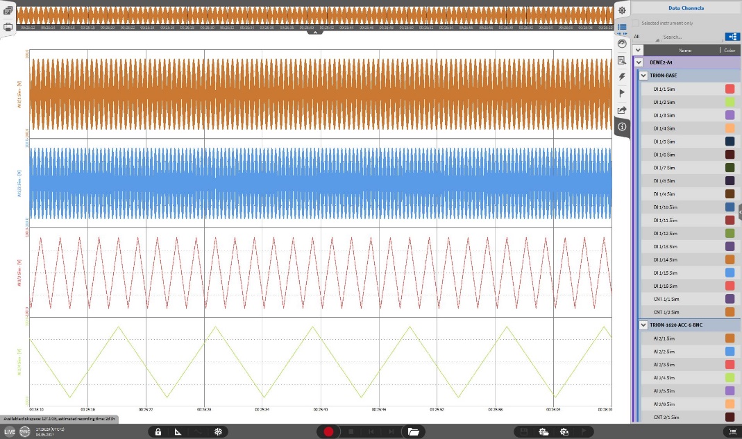
Fig. 174 Data Channels menu - quick view
A single click on the Data Channels menu button will open the quick view where the user can see the activated hardware channels (see Fig. 174). Expanding the menu to the full screen by keeping the button pressed and moving the mouse to the opposite side of the screen will open the full data channel menu that can be seen in Fig. 175. The full channel list and the connected hardware with the individual settings can be checked and manipulated here. The functionality of the individual buttons will be explained in the following section.
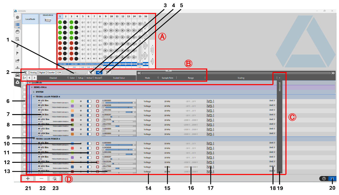
Fig. 175 Complete Data Channels menu
No. |
Name |
Description |
|---|---|---|
A - Hardware overview |
||
Quick overview of your connected TRION boards and available channels. Click on a certain channel or whole TRION board and the respective channel(s) will be highlighted in the list. |
||
B - Filter and grouping |
||
1 |
Search Filter |
Search a channel according to its name |
2 |
Channel Filter |
Filters the displayed channels according to their channel type (All, Analog, Digital, Counter, EPAD, Math, Video, Power, CAN). These channel types can also be set as favorite. Additionally it is possible to filter all channels with a specific channel tag. |
3 |
Clear Filters |
Clear active Channel and Search Filters |
4 |
Channel Grouping |
Sort the Channel list according to the connected TRION board or in an alphabetical order |
C - Channel options |
||
5 |
Change channel sorting (non- analog channels) |
When selected, non analog channels like math or statistic channels can be rearranged (see Fig. 176). |
6 |
Select button |
Select several channels in the list, i.e. for setting them active or inactive simultaneously. |
7 |
Channel Name |
Individual channel name; Can be changed individually; for additional information refer to User interface. Deleting the channel name and pressing ENTER restores the default channel name. In case a name is given twice, a warning is displayed. |
8 |
Color |
Color scheme of the channel can be changed here |
9 |
Hide button |
Hide the channels of a complete card |
10 |
Setup |
Enter the input channel setup (All channel dependent settings can be changed here). |
11 |
Active button |
Set a channel active or inactive; An active channel can be displayed in an instrument, used in a math channel and can be recorded, an inactive channel not |
12 |
Stored button |
Select whether channel data shall be stored or not when a measurement is running |
13 |
Scaled Value |
Preview of the input signal |
14 |
Mode |
Change the mode of the input channel here |
15 |
Sample Rate |
Change the sample rate here; Remark: to change the sample rate for individual channels refer to Channel-wise Sample Rate Selector. |
16 |
Range |
Change the input range of the channel here |
17 |
Scaling |
Change the channel scaling here |
18 |
Physical unit |
Physical unit of the channel, can be changed in the channel setup |
19 |
Advanced Options |
Expand the channel dependent advanced Options: Excitation, LP Filter, Coupling, Input Type, Sample Format, Sensor Offset, Baud rate, Counter_Filter, Inverted_A, ListenOnly, Source_A, Termination, Threshold |
20 |
Toggle button |
Quick access to Data channels menu; toggles between the Channel List and the previously opened menu |
D - Math options |
||
21 |
Add button |
Add a Formula, Statistics, Filter, FFT, Rosette, Power Group, Ethernet Receiver or Ethernet Sender |
22 |
Delete button |
Delete the Formula, Statistics, Filter, FFT, Rosette, Power Group, Ethernet Receiver or Ethernet Sender that is currently selected |
23 |
Create Power Group |
Create Power Group with selected channels or empty Power Group |
Note
To quickly navigate through long channel lists, use the shortcut CTRL + PAGE UP / PAGE DOWN. This function works both in full-screen view and in the compact side panel view of the channel list.
The following screenshot belongs to No. 5 in Table 10.
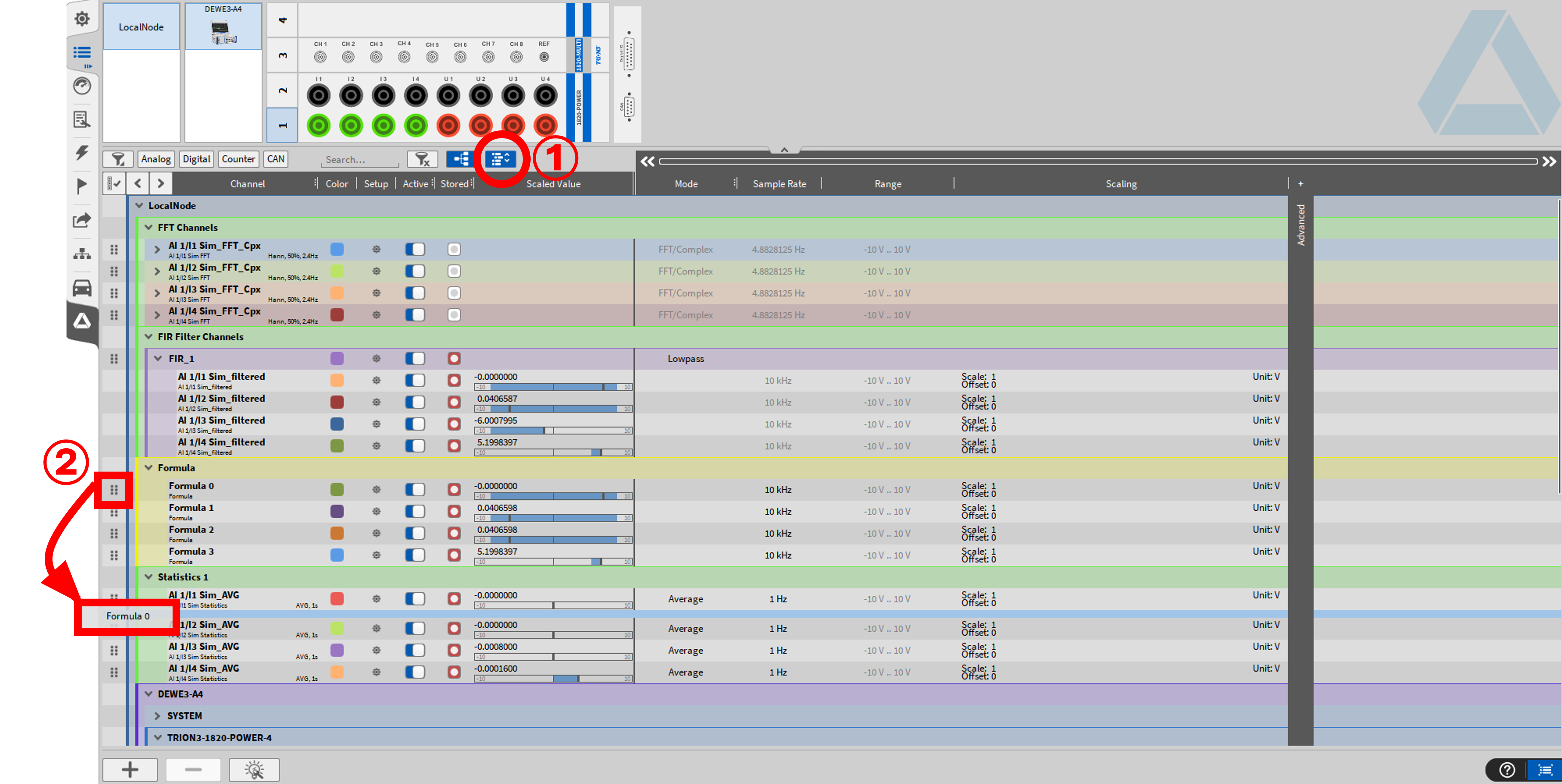
Fig. 176 Channel sorting
If a measuring card is completely folded in, as shown in Fig. 177, the slot number in which the respective measuring card is located is displayed.
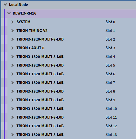
Fig. 177 Slot numbering with folded modules
Filter- and grouping options
Selecting multiple channels
Inside the Data Channels menu, the user can select multiple Input channels through various methods. With multiple channels selected, the user can address changes in Channel Settings to multiple channels at one time.
To select multiple channels:
Select a channel using the system graphic in the upper left-hand corner of the Data Channels menu
Select a check box on the left edge of the individual Data Channels menu adjacent to each individual channel
The user can also just simply click onto the channel row itself and select several channels by keeping the CTRL key pressed
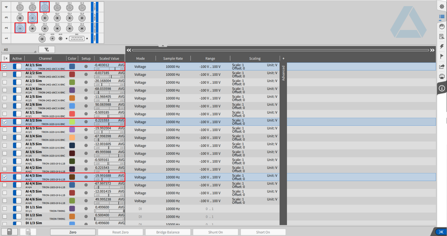
Fig. 178 Selection of several channels
Channel List filtering options
As explained in Table 10, the user can filter the channels according to their channel type or their channel name, e.g. to only show relevant channels. There are additional filtering options available which are explained in the following sections.
To get to the different filter options in the channel list, fully open the Data Channel menu.
Filtering by the Channel Type
To filter the channels by their type different buttons are shown on the upper border of the channel list, shown in Fig. 179. These buttons vary depending on the available channels, meaning only those buttons are shown, for which the according channels are really available in the channel list.
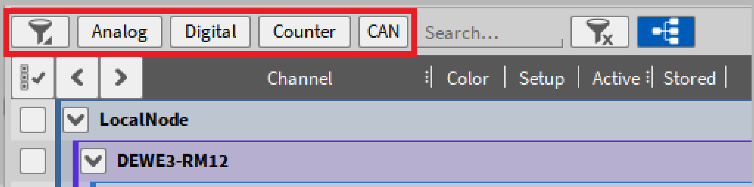
Fig. 179 Filtering by the channel type
After choosing a type the button turns blue and only the according channels are shown.
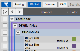
Fig. 180 Filtering by the channel type: Digital
Note
Only one channel type can be selected, therefore, it is not possible to select more buttons at the same time.
Filtering Channels by Name/Active/Mode
Another option is to filter the channels by their names or mode or just to show active channels. Those filter options are shown by 3 dots in the column header (see Fig. 181).
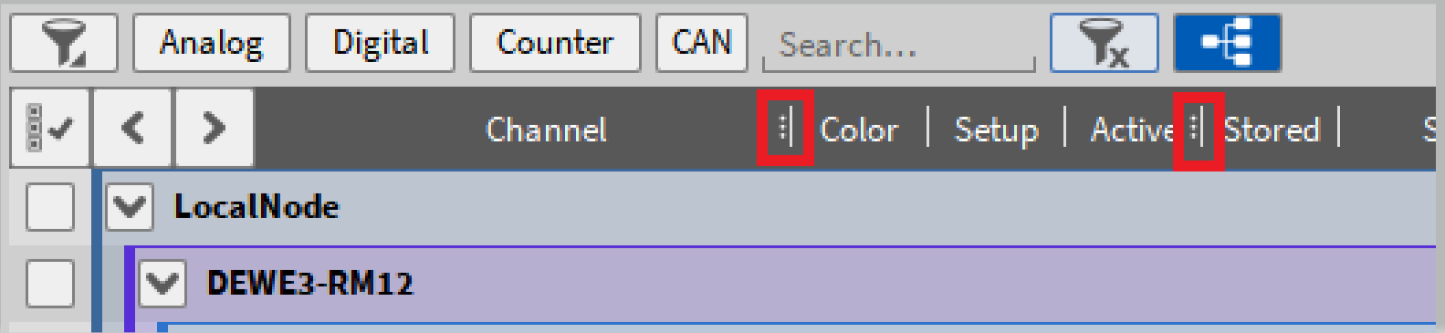
Fig. 181 Filter option available in Data Channel Menu
Fully open the Data Channels menu
Left click onto the column header opens a filter menu for: channel, active, mode
A sorting menu will appear for each filter menu, which allows the user to sort from A to Z, Z to A, by name/prefix such as AI or DI, or by true or false. Sorting by true or false will sort your channels by whether your channels or active (true) or inactive (false). The user can simply type a channel name within the menus text field. This may seem like a difficult task, but the software will automatically update the channel list as you type. Selecting a specific Mode name such as Temperature will only present the user with those specified channels.
Delete an active filter with the Clear filter button again (see ③ in Table 10)
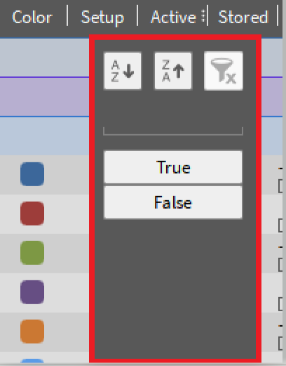
Fig. 182 Filtering by the Active Column
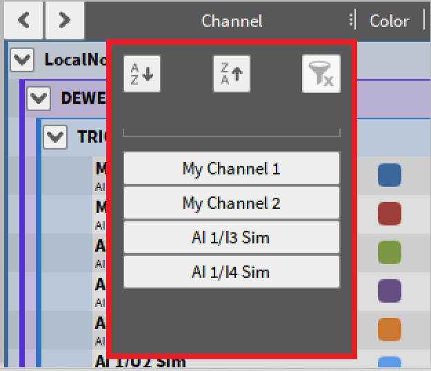
Fig. 183 Filtering by the Channel Column
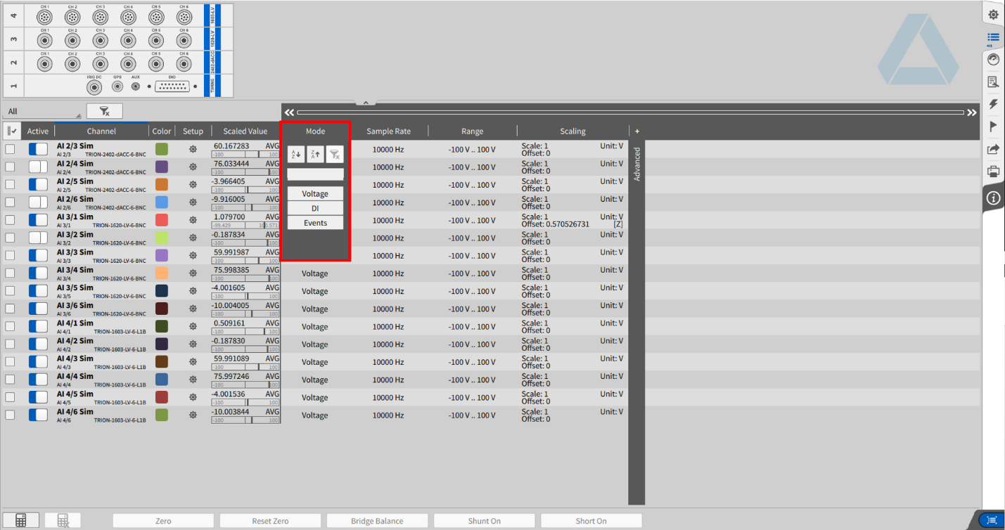
Fig. 184 Filtering by the Mode Column
Channel Tag filtering options
It is possible to define channel Tags and assign channels to them for additional grouping. This is possible in the detailed channels setup, which is accessible by clicking on the gear symbol of a channel (see ① in Fig. 185). By clicking on the Tag symbol (see ② in Fig. 185) a new window will be opened where a custom Tag name can be entered (see ③ in Fig. 185) or it is possible to select an already added channel Tag out of the list when clicking in the text field. By clicking on the “+” button next to the text field, the respective channel will be assigned to the selected Tag.
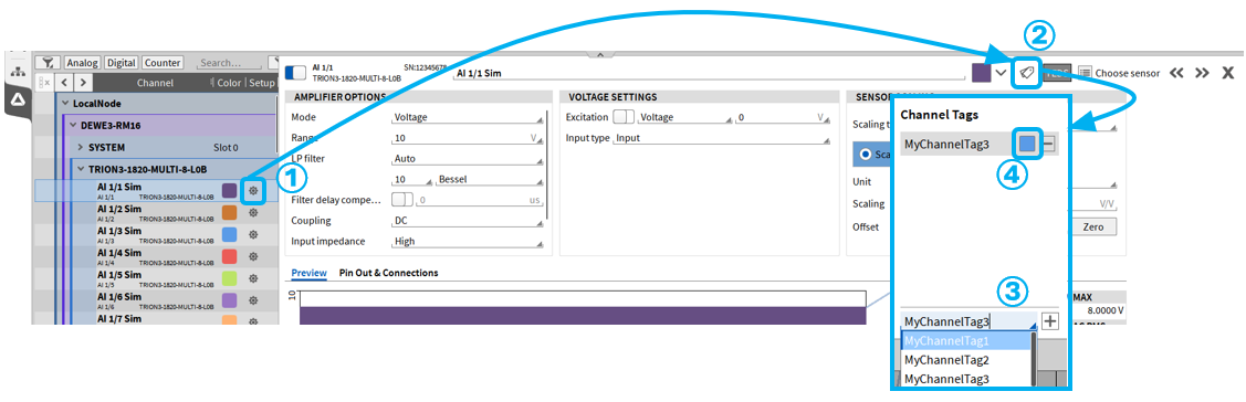
Fig. 185 Set Channel Tags for filtering
If a channel is linked to a specific Tag, it will be displayed directly in the channel list next to the name of the channel (see Fig. 186). It is also possible to set a specific color for each channel Tag (see ④ in Fig. 185). By clicking on one of the channel Tags all channels which are assigned to this Tag will be selected automatically in the channel list.
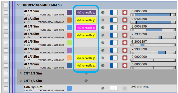
Fig. 186 Channel Tags in channel list
When at least one channel Tag has been defined an additional option for the channel Tags will be listed in the filter option section of the OXYGEN channel list (see ① in Fig. 187). After selecting a Tag, only those channels will be listed in the OXYGEN channel list, which are assigned to the respective Tag.
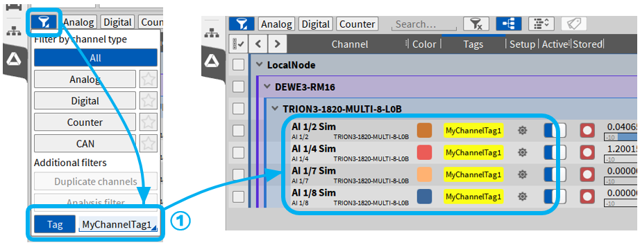
Fig. 187 Channel Tags in filter options
Changing the channel settings
It is either possible to change the channel settings in the Data Channels menu or in the individual channel setup that can be accessed via push button ⑩ (see Table 10). Additionally, settings can be copied (CTRL+C) and pasted (CTRL+V) between channels of the same type (e.g., from one CNT channel to another, or from one Analog In channel to another, etc.).
For documentation purposes, you can copy the entire channel configuration into third-party software such as Notepad, Excel, or similar tools. To do this, simply select the desired channels, press CTRL+C, and paste the configuration into the target application.
Changing the channel settings in the Data Channel menu
To change the individual channel settings in the Data Channels menu just click on the desired parameter with the left mouse button and a pop-up window will appear. If a parameter can be changed or not depends on the channel type (i.e. it is not possible to change the range of a digital channel) and the selection of the parameters depends on the TRION board (i.e. different Input Modes). For illustration, the following figures will show the different options that are available with a TRION-1620-ACC board.
Changing the channel color
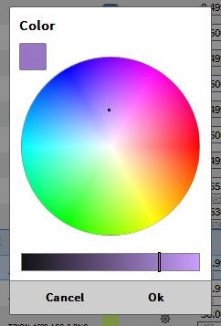
Fig. 188 Pop-up window for changing the channel color
Changing the input mode
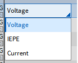
Fig. 189 Pop-up window for changing the input mode
Changing the sample rate
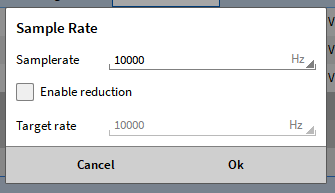
Fig. 190 Pop-up window for changing the sample rate
It is possible to change the sample rate for the whole board but also to change the sample rate channel-wise. For a detailed explanation see Sensor scaling – bridge.
Changing the input range
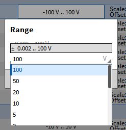
Fig. 191 Pop-up window for changing the input range
Changing the channel scaling and physical unit
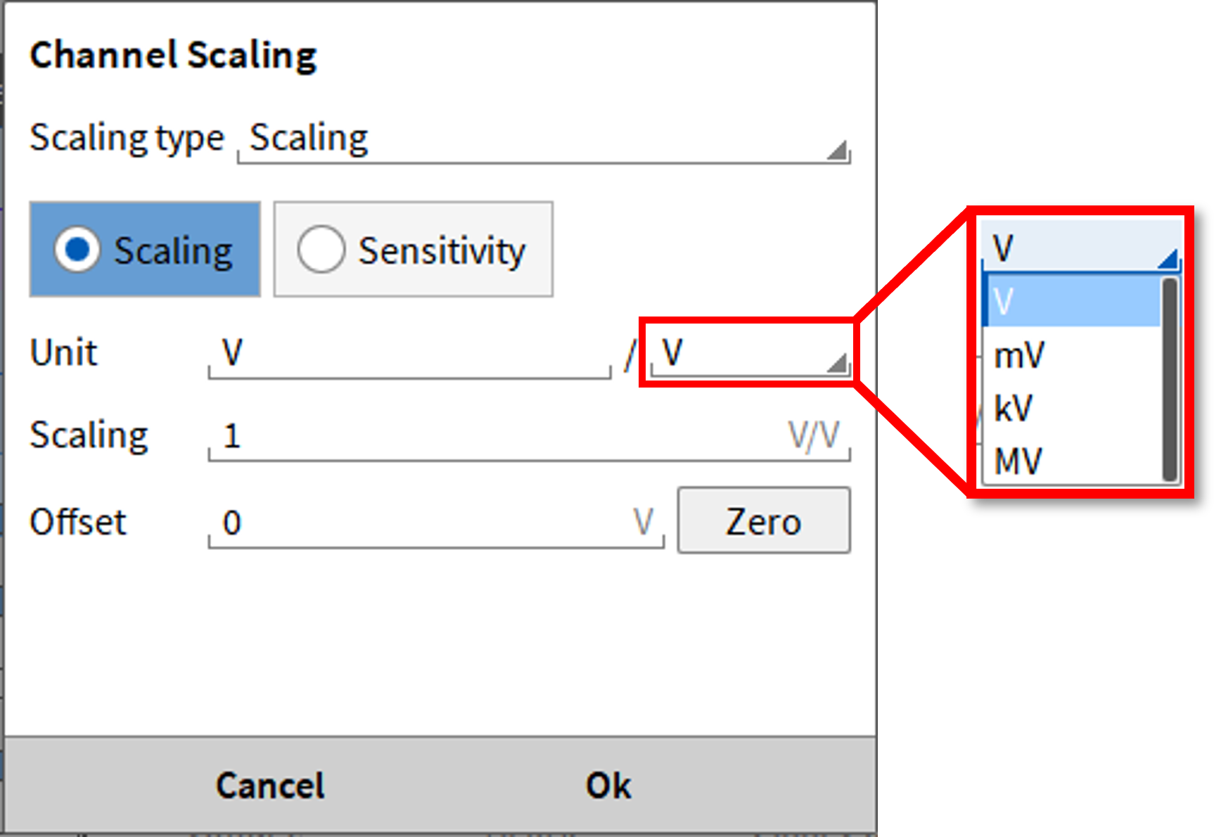
Fig. 192 Pop-up window for changing the scaling and physical unit
Zeroing an input channel
After selecting the desired channel in the list the Zero push button will appear at the lower end of the Data Channels menu:
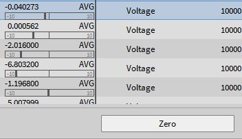
Fig. 193 Zeroing an input channel
Changing the sensitivity
Also available in the Channel Scaling pop-up window:
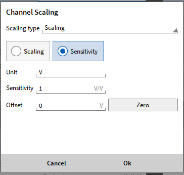
Fig. 194 Pop-up window for changing the sensitivity
Changing the 2-point-scaling
Also available in the Channel Scaling pop-up window:
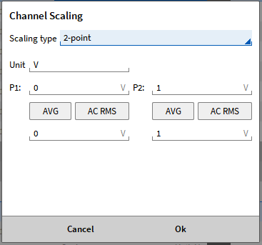
Fig. 195 Pop-up window for changing the 2-point-scaling
By clicking the AVG or the ACRMS button, a direct measurement point at the current instant of time can be used. A time window of 1 s into the past is used.
It is also possible to perform AVG & ACRMS calibration for multiple channels at the same time by selecting multiple channels in the channel list. By clicking on the scaling option in the channel list, the 2-point scaling window opens. By clicking on the AVG or ACRMS button, the respective value is automatically used for each selected channel individually (see Fig. 196).
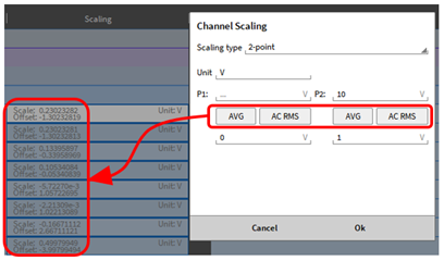
Fig. 196 AVG & ACRMS calibration for multiple channels
Applying table scaling
Also available in the Channel Scaling pop-up window:
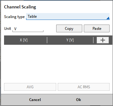
Fig. 197 Pop-up window for applying table scaling
Applying polynomial scaling
Also available in the Channel Scaling pop-up window:
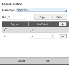
Fig. 198 Pop-up window for applying polynomial scaling
Changing the bridge scaling settings
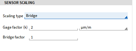
Fig. 199 Scaling setting for bridge mode
For more details about the sensor scaling for the bridge mode see Sensor scaling – bridge.
Changing the LP filter (Expand advanced settings)
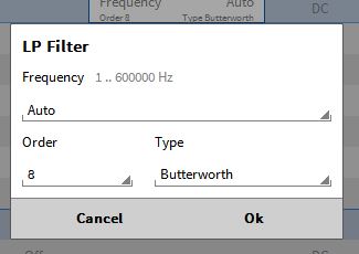
Fig. 200 Pop-up window for changing the LP filter
Note
When the sample rate is changed an appropriate filter will be selected automatically (Auto-mode).
Changing the coupling mode (Expand advanced settings)
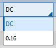
Fig. 201 Pop-up window for changing the coupling mode
Changing the bit resolution (Expand advanced settings)
Can only be changed for the whole board and not for single channels:
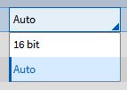
Fig. 202 Pop-up window for changing the bit resolution
Setting a sensor specific delay
For analog inputs it is possible to define a sensor specific delay in the range of 0-500ms
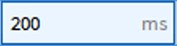
Fig. 203 Pop-up window for compensating the sensor delay
The delay (of the sensor) on this incoming signal is then compensated by the specified time (see Fig. 204).
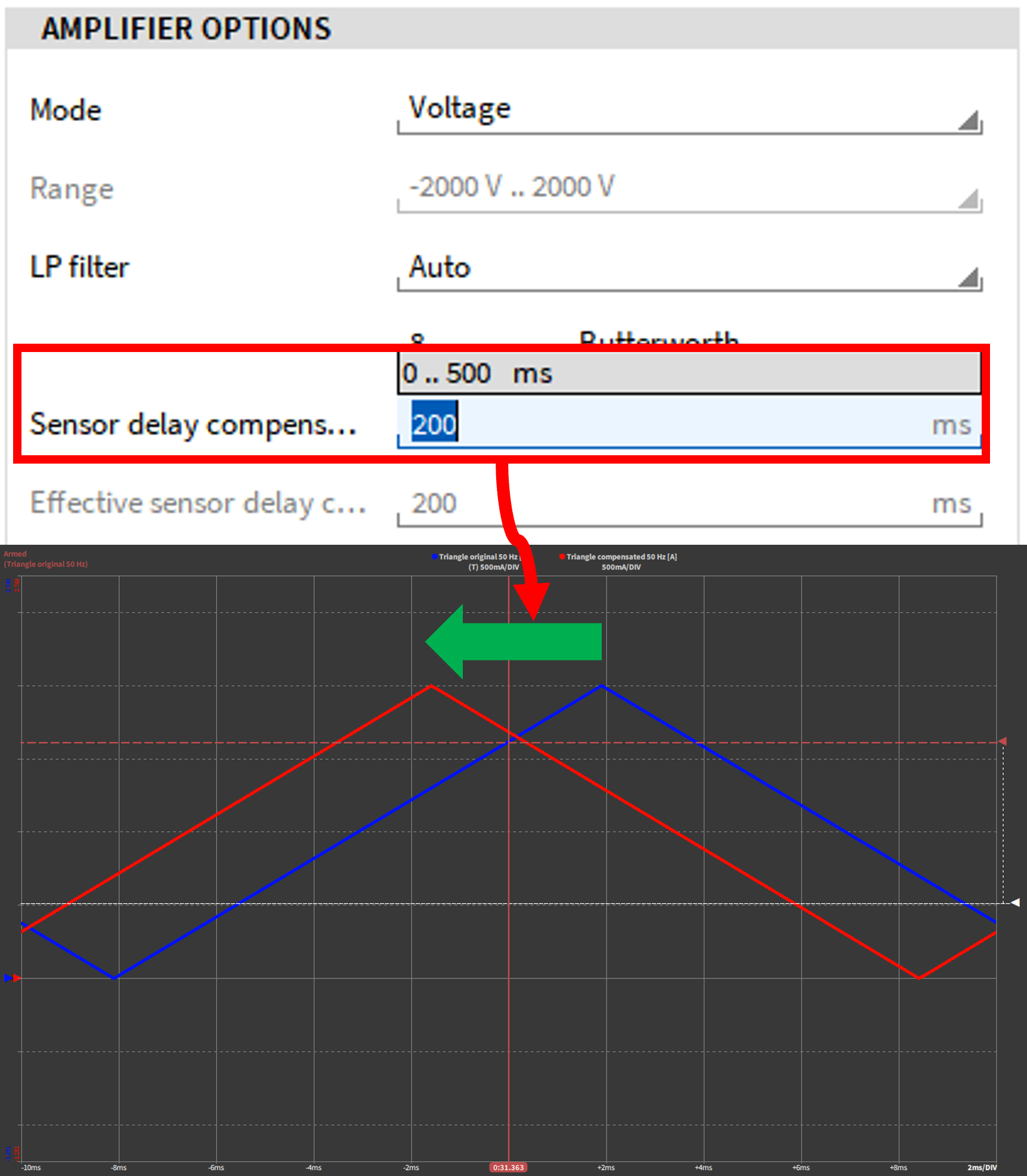
Fig. 204 Compensating the sensor delay
The effective sensor delay is calculated based on the sample rate and always rounded off. For example, at a sample rate of 100 Hz and a sensor delay of 99 ms the effective sensor delay is set to 90 ms.
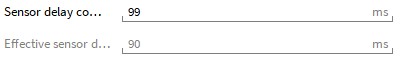
Fig. 205 Effective sensor delay which can be applied
Channel-wise Sample Rate Selector
To change the sample rate of whole module simply click on one of the sample rates of a channel of that module and select the desired sample rate from the Sample rate drop-down list (see Fig. 206).
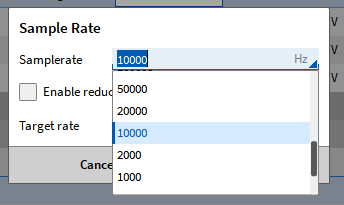
Fig. 206 Selection of the sample rate of a TRION module with the drop-down list
To change the sample rate just for an individual channel, click on the Enable reduction button in the Sample Rate window (see Fig. 207). The target rate can then be selected from the drop-down list. There is a selection of different sample rates available for an individual channel as integer divisors down to 1/10000th of the sample rate of the module. It is not possible to enter a sample rate, only to select one from the drop-down list.
For example, if the sample rate of the module is selected as 200 kHz, the smallest available sample rate for a channel on that module is 20 Hz.
Note
The smallest available reduction is 1 Hz. If the sample rate of the module is 100 Hz, the smallest reduction for a channel is 1 Hz.
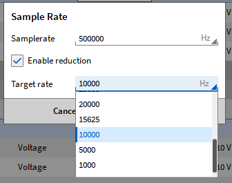
Fig. 207 Selection of a sample rate for an individual channel
In case the sample rate of the module will be changed, whenever a reduction is active, the target rate stays the same if it is still an integer divisor of the new sample rate of the module. This also means that only a reduction of the module sample rate is possible.
Example The sample rate of the module is set to 500 kHz and Channel 2 is set to a reduced sample rate of 20 kHz. The sample rate of the module is now changed to 100 kHz, and the target rate of Channel 2 stays at 20 kHz, since this is also an integer divisor of 100 kHz.
In case the target rate does not fulfill this requirement when the sample rate of the module is changed, if i.e. the sample rate is smaller than the reduced rate of a channel, the effective rate is shown in red below the target rate seen in Fig. 208. The effective rate is chosen to be as close as possible to the original selected target rate, which is still possible with the new sample rate of the module. With the Accept button this effective rate will be used as the new target rate of the channel.
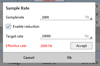
Fig. 208 Effective sample rate when changing the sample rate of the module
In case this suggested effective rate is not accepted by clicking the button, the effective rate is shown in red in the channel list (see Fig. 209). The originally selected target rate is shown in brackets below. Even though the effective rate was not accepted, it will still be used as new target rate for this channel. The red marking solely serves as an indication for this.
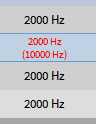
Fig. 209 Not accepted effective rate as reduced sample rate in the channel list
Information
The channel-wise sample rate selector is also applicable with formula channels
The frequency of the AUTO-Filter will be adjusted automatically with the new sample rate
Working principle
This chapter shortly explains the working principle behind the channel-wise sample rate selector. The samples are physically sampled with the set sample rate, which is defined in the channel list (red box in Fig. 210). If the reduction is enabled the user can set a reduced sample rate (blue box in Fig. 210) which is converted to an integer divider in the background and unnecessary samples are skipped
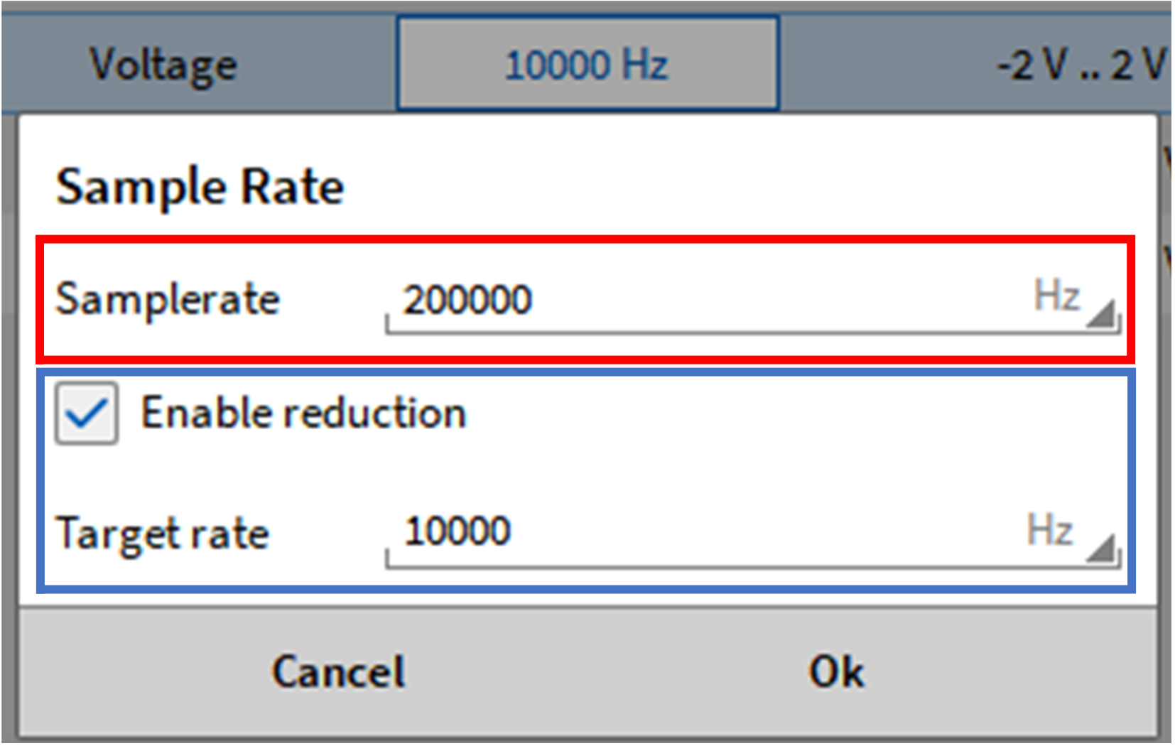
Fig. 210 Channel-wise sample rate settings
If the filter settings are set on AUTO, the filter is adjusted according to the target sample rate, therefore, the user must not worry about aliasing. In the exemplary settings above, the filter would be set automatically to 3333.3 Hz for this channel. However, the user can override the filter settings if needed.
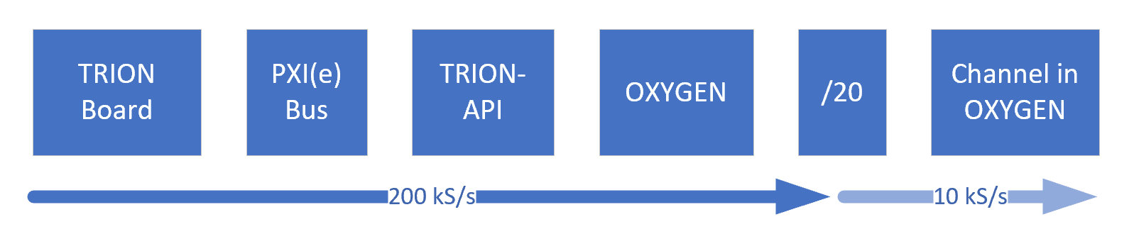
Fig. 211 Working principle for the channel-wise sample rate reduction
Example
In Fig. 212 exemplary signals with and without sample rate reduction and with different filter settings can be seen. The different signals have the following settings:
Blue signal - Sample rate: 200 kS/s - Filter setting: AUTO
Red signal - Reduced sample rate: 10 kS/s - Filter setting: AUTO
Green signal - Reduced sample rate: 10 kS/s - Filter setting: 66666.6 Hz
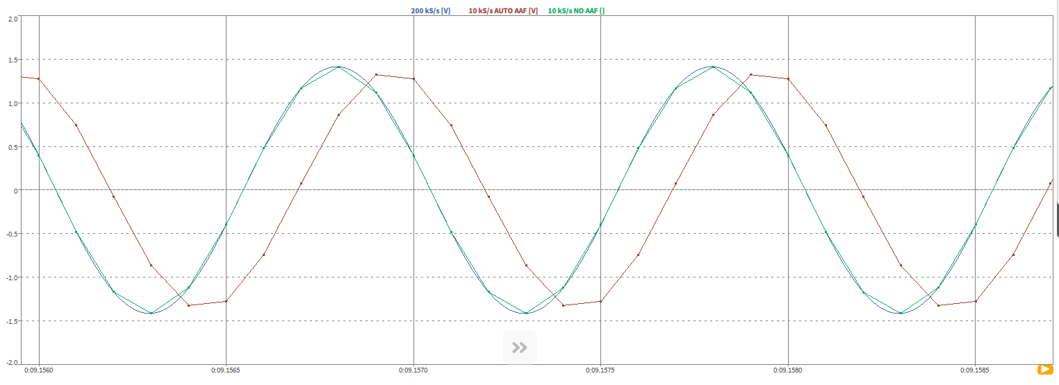
Fig. 212 Channel-wise sample rate reduction with example signals
The red signal is phase-shifted due to the anti-aliasing filter, which is automatically set to 3333.3 Hz. The green signal also has a reduced sample rate and a manual set filter, according to the auto filter setting of the blue signal. Therefore, those two signals are not phase-shifted. In this case, the user must be aware of aliasing.
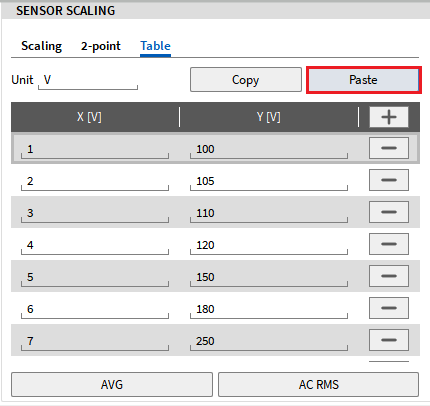
Table scaling
OXYGEN offers the possibility to apply non-linear scaling in form of a table for non-linear sensors. This can be done in the data channel menu but also in the channel settings of an individual channel.
Following options are available:
The unit can be specified
Individual points to specify x- and y-values can be added by clicking on the + button (see Fig. 210)
A point can be removed by clicking on the – button (see Fig. 211)

Fig. 213 Table scaling – add point to specify x- and y-value
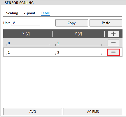
Fig. 214 Table scaling – delete point
By clicking the AVG or the AC RMS button, a direct measurement point at the current instant of time can be added to the table. A time window of 1s into the past is used.
A table can also be copied from another source, e.g. Excel and pasted with CTRL+V or the Paste button into the table scaling menu. Likewise, the table can be copied using CTRL+C or the Copy button and pasted into e.g. Excel (see Fig. 212).
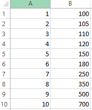 →
→ 
To copy and paste a whole table from one channel to another the Copy button in channel 1 can be used. After entering the channel settings of channel 2, the Paste button can simply be clicked on, and the table will also be applied here.
Note
For a valid scaling, at least two points have to be added, otherwise an error message will appear.
If duplicate x-values exist in the table, an error message will appear.
If a value is out of the defined table range the scaling will be extrapolated.
Linear interpolation is applied between the table points.
The x-values do not necessarily have to be entered from lowest to highest value, since the table will be sorted when leaving and entering the menu again.
As it is also noted in Selecting multiple channels, the whole channel settings, including the table scaling, can be copied and pasted between different channels using CTRL+C and CTRL+V.
Polynomial scaling
OXYGEN offers the possibility to apply non-linear scaling in form of a polynomial for non-linear sensors. This can be done in the data channel menu but also in the channel settings of an individual channel. The following options are available (see Fig. 215):
The unit can be specified.
A polynomial coefficient can be added by clicking on the + button.
A polynomial coefficient can be deleted by clicking on the – button.
By clicking on the Copy button the table can be copied and pasted in e.g. Excel or a third party program.
The polynomial scaling can also be pasted from another source, e.g. Excel by clicking on the Paste button or with the shortcut CTRL+V
Each coefficient must be defined. In Fig. 215 and Fig. 216 the following polynomial is represented:
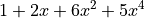
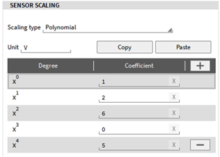
Fig. 215 Polynomial scaling
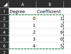
Fig. 216 Copying of a table for the polynomial scaling in OXYGEN
Enum scaling
The so-called enum scaling or enum label editor is available in the scaling section of the channel settings for some defined channels. With the enum scaling a text label can be defined for a specific, unique signal value. The text label is then shown in the digital instrument and as labels in the recorder (if activated, see Instrument properties), whenever the signal value takes on the specified value, see Fig. 219. The following channels support enum scaling:
CAN channels: If the DBC file already includes an enumeration it can be parsed. The enumeration can be edited in the enum scaling editor.
Flexray and ARXML channels: Parsing of enum data is not supported
Ethernet receiver channels
IMU (ADMA & OxTS) channels: Enum data is not stored in the channel definition
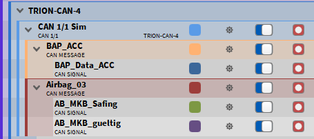
Fig. 217 Enum Scaling of a CAN channel
In the enum scaling editor new labels can be created by clicking on the + button, and deleted by clicking on the – button. The table can be copied (Copy button) and pasted into another program. An existing table can also be pasted from another source into OXYGEN (Paste button).
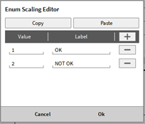
Fig. 218 Enum Scaling Editor
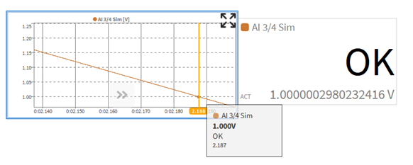
Fig. 219 Enum Scaling - display in the digital instrument and as label in the recorder
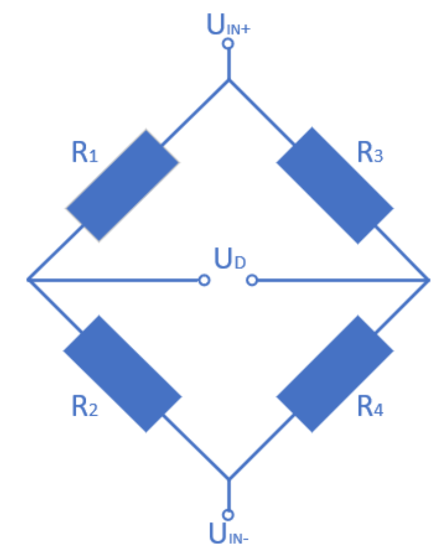
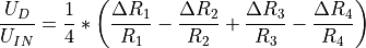
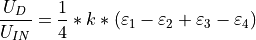
Sensor scaling – bridge
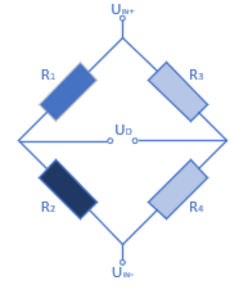
The following section gives a small overview about the scaling setting for different bridge configurations. For a detailed explanation about this topic refer to further literature.
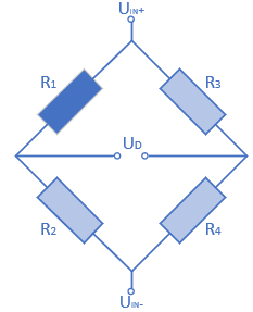
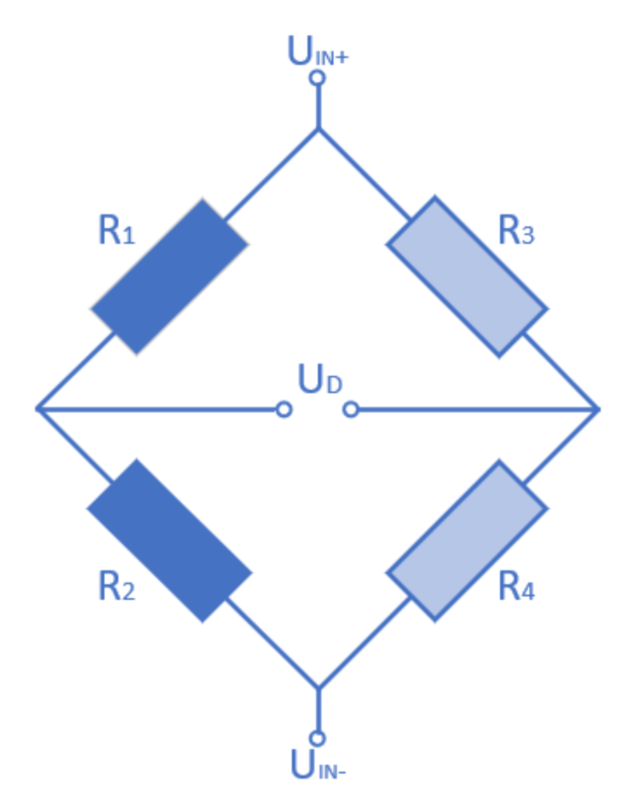
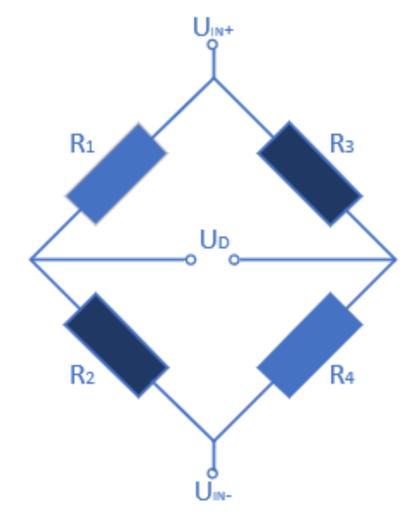
The following definitions are used for the equations:
Ri … Strain gage resistor of the bridge
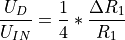
UD … Bridge output voltage
UIN … Bridge supply voltage
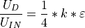
ε … Elongation
k … Bridge factor
ν … Poisson’s ratio
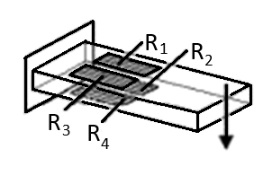
Quarter bridge
Used to measure tension and compression
Schematic |
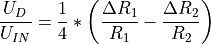
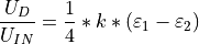
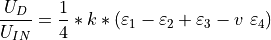
UD / UIN equation |
Bridge factor |
Linearity |
Active strain gauges |
|---|---|---|---|---|
|
|
1 |
No |
One active strain gauge (R1) |

Half bridge
Used to measure bending
Schematic |
UD / UIN equation |
Bridge factor |
Linearity |
Active strain gauges |
|---|---|---|---|---|
|
|
2 |
Yes |
Two active strain gauges (R1 and R2). The elongation of R1`and R:sub:`2 must be the same but opposite in sign, i.e. one strain gage can be put on top of a beam and the other on the bottom. |
Used to measure tension and compression
Schematic |
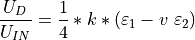
UD / UIN equation |
Bridge factor |
Linearity |
Active strain gauges |
|---|---|---|---|---|
|
|
(1 + v) |
No |
Two active strain gauges (R1 and R´2). 1x longitudinal elongation / 1x transverse elongation. One strain gauge lies in principal and the other in transverse direction. |
Full bridge
Used to measure bending
Schematic |
UD / UIN equation |
Bridge factor |
Linearity |
Active strain gauges |
|---|---|---|---|---|
|
|
2 x (1 + 1) |
Yes |
|
Used to measure tension and compression
Schematic |
UD / UIN equation |
Bridge factor |
Linearity |
Active strain gauges |
|---|---|---|---|---|
|
|
2 x (1 + v) |
No |
Four active strain gauges (R1, R2, R3 and R4); 1x longitudinal elongation, 2x transverse elongation. One pair of strain gauges lies in principal and the other pair in transverse direction. |
Changing the channel settings in the channel setup
All channel settings (except the sample rate and the bit resolution) can also be changed in the individual Channel Setup (see Fig. 220) which can be accessed via push button ⑪ (see Fig. 175 or Table 10).
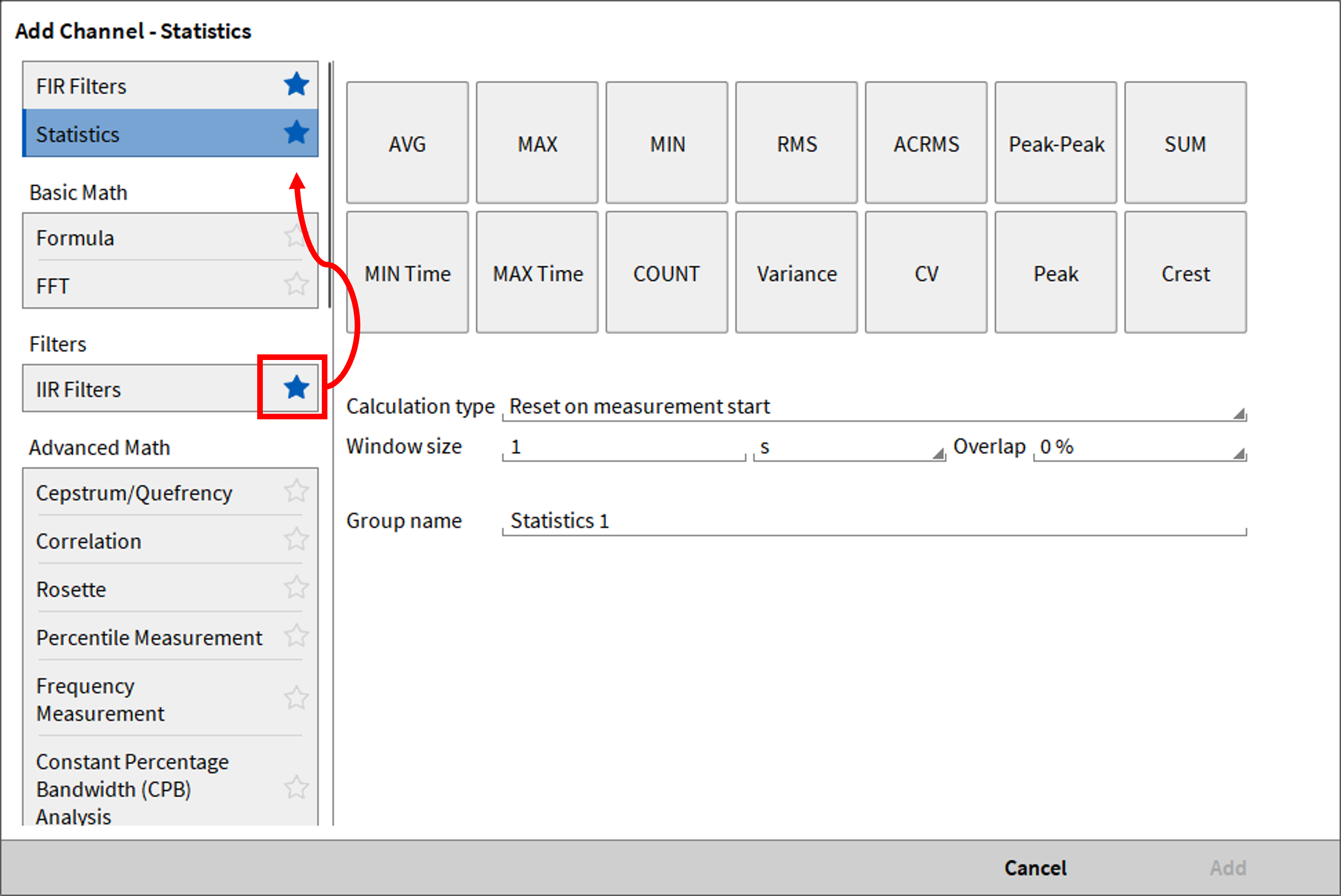
Fig. 220 Channel setup of a TRION3-1820-MULTI channel
The main advantage compared to the parameter manipulation in the Data channels menu is that a wide preview window is available. With that, the user can see the affection of different parameter changes (i.e. range and scaling) on the input signal in real time. To swap between the channel setups of different channels use the arrows (<< >>) in the upper right corner and to close the channel setup use the X next to the arrows. In addition, depending on the mode, a connector pinout is available.
Current measurement using TRION modules
Different TRION modules can be used for current measurement. Current signals can be connected directly to TRION-1603-LV-6-L1B, TRION-1620-LV-6-L1B and TRION-1620-ACC-6-L1B modules and measure the current via an integrated 10 Ω shunt resistor.
Other modules can also be used for current measurements but need an external shunt resistor to support this functionality. These modules are the following: TRION-1603-LV-6-BNC, TRION-1620-LV-6-BNC, TRION-1620-ACC-6-BNC, TRION-1820-dLV, TRION-1600-dLV and TRION-2402-x. The TRION-1820-PA module is excluded from this consideration.
Modules that require an external shunt resistor for the current measurement contain a predefined shunt resistor selection in the Channel List (see Fig. 221) if Current Amplifier Mode is selected.
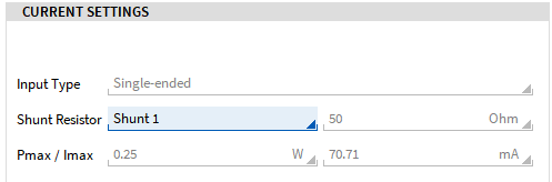
Fig. 221 External Shunt resistor selection in the Channel Setup
From the technical point of view, the current measurement via an (external) shunt resistor is the measurement of the potential difference that is caused by the current on the shunt resistor.

The voltage U is measured, the resistance R is known and therefore the Current I can be determined. Thus, if the current is measured via an external shunt, a voltage signal representing the potential difference caused by the current on the external shunt is provided to the TRION-module. This voltage is rescaled to the current again by using the formula above. This rescaling is done by OXYGEN. Therefore, the resistance must be known and can be selected in the drop-down list from Fig. 221.
For sure, any shunt resistor can be used and not the ones contained in the drop-down list. If a shunt is used whose resistance is not contained in the list, the rescaling of the voltage signal representing the current can be done manually in Voltage Amplifier mode proceeding the following steps:
Set the Amplifier Mode to Voltage (see Fig. 222):
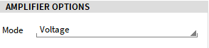
Fig. 222 Voltage measurement mode
Change the Unit to A (Ampere) and enter the resistance of the shunt resistor as Scaling factor, i.e. 50 Ω (see Fig. 223).
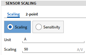
Fig. 223 Entering the shunt resistance as scaling factor
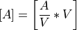
With these settings, the rescaling of the voltage signal to the represented current is done in the same manner as in Current mode with the corresponding shunt resistor selected in the drop-down list. Thereby, the voltage signal is multiplied with the entered Scaling factor and the result of this equation is the corresponding current:

Considering the physical units of this equation will clarify that:
If a TRION module with integrated 10 Ω shunt is used for the current measurement, this consideration can be neglected! This applies only for current measurements via external shunt resistors.
Software channels
In addition to hardware channels (analog, digital, CAN, counter, etc.), OXYGEN also allows creating software channels (also referred to as math channels). Software channels offer various functions such as basic and advanced math, analysis tools, software filters, and data input/output features. All available software channels are described in detail in the following sections.
Working with Software Channels
Creating a new software channel (see Fig. 224):^
Click the [+] button in the lower-left corner.
A pop-up window opens. Select the desired software channel.
Configure the channel-specific settings if required.
Press Add to create the channel.
Created channels will show up in their respective channel group in the Data Channels menu.
Note
Some software channels (e.g., FFT) require selecting the input channels before pressing Add. If applicable, this is mentioned in the respective software channel description.
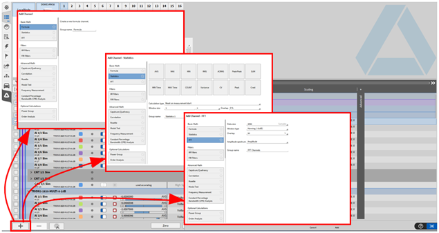
Fig. 224 Creation of a math channel
Deleting existing software channels (see Fig. 225)
Select the channel(s) to be removed.
Click the Delete button.
A confirmation window will pop up to prevent accidental removal of channels. Confirm the deletion in the pop-up window.
Note
The confirmation window pop-up can be enabled/disabled within the Advanced Settings in the OXYGEN Setup menu.
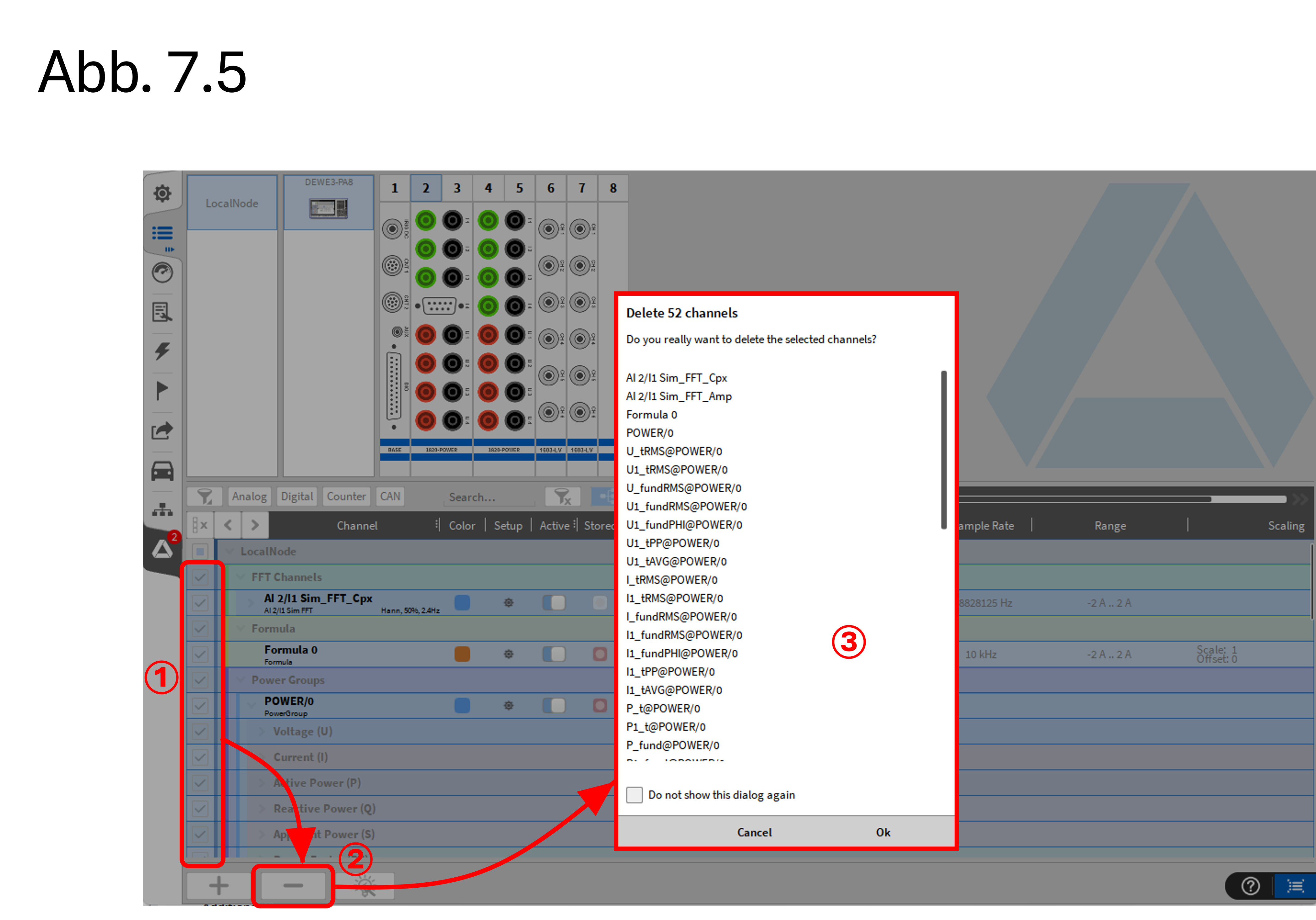
Fig. 225 Deleting software channels
Favorites and Quick Search
Specific software channels can be quickly located by using the search function or by marking them as favorites (see Fig. 226). Marked favorites are automatically moved to the top of the list for faster access. When a favorite is unmarked, it returns to its default position in the list. When one or more software channels are marked as favorite, the power button shows the favored (starred) software channels instead.
Fig. 226 Add favorites
Basic math
Formula channel
To create Formula channels, click on the [+] button in the lower-left corner of the Data Channels menu (see Working with Software Channels) and select Formula. In the Add Channel pop-up, it is possible to assign a group name and define the number of formula channels to be created:
Group name: use to organize multiple formulas under one group in the channel list.
Channels: specify how many formulas to create — up to 100 formula channels can be added at once
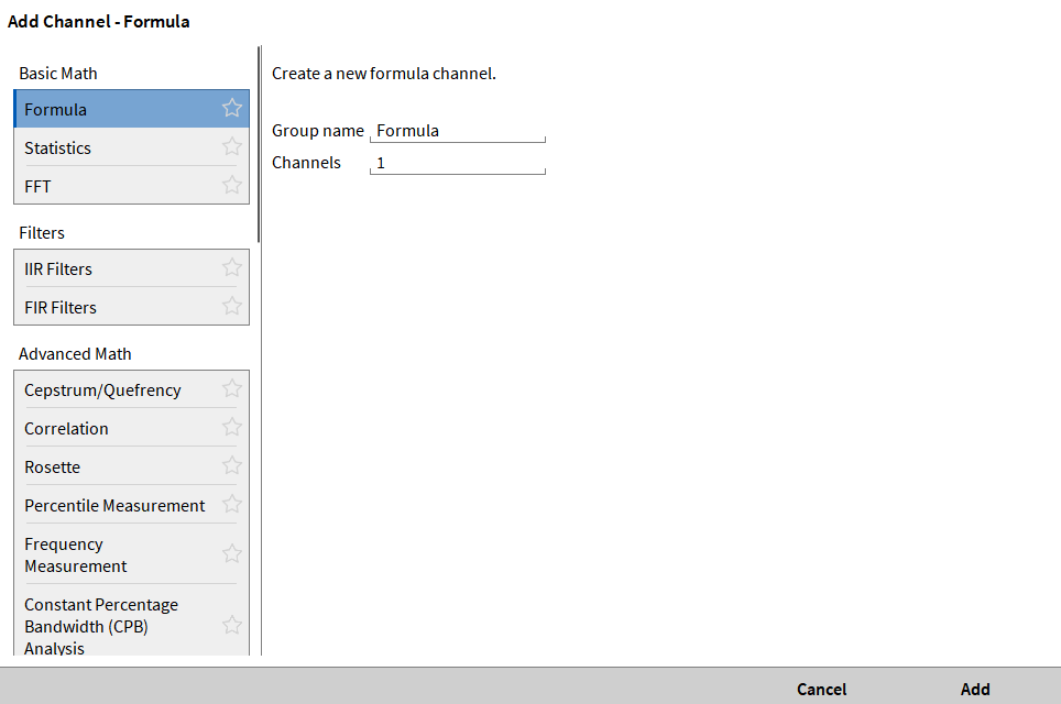
Fig. 227 Pop-up window for creating a Formula channel
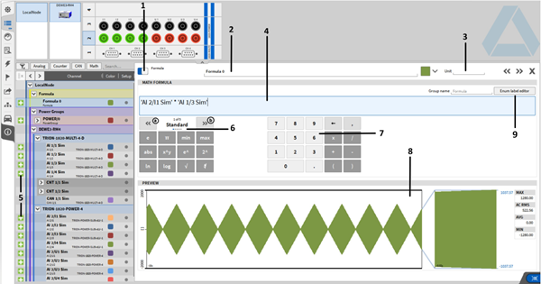
Fig. 228 Formula channel setup - overview
No. |
Name |
Description |
|---|---|---|
1 |
Active button |
Setting a channel active or inactive; An active channel can be displayed in an instrument, used in a math channel, and can be recorded, an inactive channel not |
2 |
Channel name |
Individual channel name; Can be changed individually |
3 |
Physical unit |
Physical unit of the channel, can be changed in the channel setup |
4 |
Command line |
Type your desired formula here |
5 |
Add button |
Adds the individual channel to the command line; Channels can be added to the command line by drag and drop, too |
6 |
Functions |
Available mathematical and logical functions can be selected here. Using the back (a) and forward (b) buttons the user can swap between Standard, Trigonometric, Logic and Miscellaneous functions. For a description and the correct syntax of the individual functions, refer to Mathematical and logical functions. |
7 |
Keys and Operators |
Numerical pad and mathematical operators; Can also be entered via the keyboard. |
8 |
Preview window |
Real Time preview of the calculation |
9 |
Enum label editor |
Enables displayed text labels for set values of this formula. Logic operations are recommended for non-digital channels. |
Note
It is possible to assign channels with different sample rates to one formula channel. The sample rate of the formula channel will be set to the highest input channel sample rate. The samples of channels with lower sample rates will not be interpolated, but the last value will be repeated according to the fastest sample rate until the channel is updated.
Mathematical and logical functions
Function |
Description |
Syntax |
|---|---|---|
e |
Euler’s number |
e |
π |
Constant Pi |
pi |
min |
Minimum of up to 128 values |
min(x,y…n) |
max |
Maximum of up to 128 values |
max(x,y…n) |
abs |
Absolute value |
abs(value) |
x^y |
Exponential function with arbitrary basis |
pow(x,y) |
e^ |
Exponential function with basis e |
exp(x) |
2^ |
Exponential function with basis 2 |
exp2(x) |
ln |
Natural logarithm to basis e |
ln(x) |
log |
Common logarithm to basis 10 |
log(x) |
√ |
Square root |
sqrt(x) |
|
Cube root |
cbrt(x) |
![\sqrt[3]{}](../_images/math/5772fde5782133fe11cd316431804c2a68cc1c6b.png)
Function |
Description |
Syntax |
|---|---|---|
sin |
Sinus based on sin(w*t+phi), e.g. “2*pi*time+pi/180*5” |
sin(x) |
asin |
Arc sine |
asin(x) |
sinh |
Hyperbolic sine |
sinh(x) |
asinh |
Arc hyperbolic sine |
asinh(x) |
cos |
Cosine |
cos(x) |
acos |
Arc cosine |
acos(x) |
cosh |
Hyperbolic cosine |
cosh(x) |
acosh |
Arc hyperbolic cosine |
acosh(x) |
tan |
Tangent |
tan(x) |
atan |
Arc tangent |
atan(x) |
tanh |
Hyperbolic tangent |
tanh(x) |
atanh |
Arc hyperbolic tangent |
atanh(x) |
Function |
Description |
Syntax |
|---|---|---|
< |
If ‘value1’ is less than ‘value2’, the result is 1.0 else 0.0 |
value1 < value2 |
≤ |
If ‘value1’ is less than or equals ‘value2’, the result is 1.0 else 0.0 |
value1 <= value2 |
> |
If ‘value1’ is greater than ‘value2’, the result is 1.0 else 0.0 |
value1 > value2 |
≥ |
If ‘value 1’ is greater than or equals ‘value 2’, the result is 1.0 else 0.0 |
value1 >= value2 |
= |
If ‘value 1’ equals ‘value 2’, the result is 1.0 else 0.0 (Two NaNs do not compare equal |
value1 == value2 |
≠ |
If ‘value 1’ is different than ‘value 2’, the result is 1.0 else 0.0 |
value1 != value2 |
and |
Logic and: value1 != 0.0 and value2 != 0.0 → 1.0 value1 = 0.0 and value2 != 0.0 → 0.0 value1 != 0.0 and value2 = 0.0 → 0.0 value1 = 0.0 and value2 = 0.0 → 0.0 |
value1 and value2 |
or |
Logic or: value1 != 0.0 or value2 != 0.0 → 1.0 value1 = 0.0 or value2 != 0.0 → 1.0 value1 != 0.0 or value2 = 0.0 → 1.0 value1 = 0.0 or value2 = 0.0 → 0.0 |
value1 or value2 |
not |
Logic negation: If value = 0.0, the result is 1.0, else 0.0 |
not value |
if |
If condition is true, the result is ‘true_val’, otherwise ‘false_val’ |
if(condition,true_val,false_val) |
isnan |
If value is NaN, result is 1.0, 0.0 otherwise |
isnan(value) |
Function |
Description |
Syntax |
|---|---|---|
ecnt1 |
Count number of edges on condition; condition is mandatory, rearm and reset parameter optional |
ecnt(cond,rearm,reset) |
hold2 |
Hold value at trigger condition; value and condition parameters are mandatory, init and rearm optional |
hold(value,cond,init,rearm) |
stopwatch3 |
Measure the timespan between two conditions in seconds; start and stop condition is both mandatory, reset is optional; if the reset is not specified, the stopwatch-function holds the value at the stop_cond and is retriggered at every new start_cond. |
stopwatch(start_cond,stop_cond, reset) |
measdiff4 |
Measure the value difference of one channel between two conditions |
measdiff(val,cond1,cond2) |
period5 |
Measure the period duration in seconds between consecutive conditions with optional rearm condition |
period(cond,rearm) |
dutycycle6 |
Measure the dutycycle (from 0 to 1) between consecutive conditions with optional rearm condition |
dutycycle(cond,rearm) |
edge7 |
Generate positive edge on cond with rearm condition |
edge(cond,rearm) |
Legend to Table 20
1 For a detailed description of the ecnt-funtion, refer to Edge-count function (ecnt).
2 For a detailed description of the hold-function, refer to Hold function (hold).
3 For a detailed description of the stopwatch-function, refer to Stopwatch function (stopwatch).
4 For a detailed description of the measdiff-function, refer to Measdiff function (measdiff).
5 For a detailed description of the period-function, refer to Period function (period).
6 For a detailed description of the dutycycle-function, refer to Dutycycle function (dutycylce).
7 For a detailed description of the edge-function, refer to Edge function (edge)
Function |
Description |
Syntax |
|---|---|---|
rmin1 |
Measure rolling overall minimum of a channel during a measurement with optional reset condition |
rmin(value,reset) |
rmax1 |
Measure rolling overall maximum of a channel during a measurement with optional reset condition |
rmax(value,reset) |
ravg1 |
Measure rolling overall average of a channel during a measurement with optional reset condition |
ravg(value,reset) |
rrms1 |
Measure rolling overall RMS of a channel during a measurement with optional reset condition |
rrms(value,reset) |
rsum1 |
Measure rolling overall sum of a channel during a measurement with optional reset condition |
rsum(value,reset) |
racrms1 |
Measure rolling overall ACRMS of a channel during a measurement with optional reset condition; Not included in the selection and must be typed manually |
racrms(value,reset) |
rp2p1 |
Measure rolling overall Peak-to-Peak of a channel during a measurement with optional reset condition; Not included in the selection and must be typed manually |
Rp2p(value,reset) |
Legend to Table 21
1 For a detailed description of the rolling-overall-functions, refer to Rolling-overall-functions
Function |
Description |
Syntax |
|---|---|---|
time1 |
Returns the elapsed time since acquisition (re)start in seconds |
time |
mtime1 |
Returns the elapsed time since measurement star in seconds |
mtime |
scnt1 |
Counts the number of samples since acquisition (re)start |
scnt |
sr1 |
Returns the Sample Rate in Hz |
sr |
dim |
When multiplied to an array channel x * dim, the output shows the current index of the bin. [1,2…n]. For scalar the index is 0. |
dim |
noise |
Noise(x), random number [-x … x] |
noise(x) |
chirp |
Creates a chirp signal with frequency from f0 to f1 within d seconds. |
chirp(f0, f1, d) |
sin wave |
Creates a sinus wave with frequency f and optional phase phi. By default, a phase shift of 0 rad is applied. |
sinwave(f,phi) |
cos wave |
Creates a cosines wave with frequency f and optional phase phi. By default, a phase shift of 0 rad is applied. |
coswave(f,phi) |
saw wave |
Creates a saw wave with frequency f and optional phase phi. By default, a phase shift of 0 rad is applied. |
sawwave(f,phi) |
tri wave |
Creates a triangle wave with frequency f and optional phase phi. By default, a phase shift of 0 rad is applied. |
triwave(f,phi) |
pulse wave |
Creates a rectangle wave with frequency f , duty cycle d and optional phase phi. By default a phase shift of 0 rad is applied. |
pulsewave(f, d, phi) |
1A channel to which the function refers must be specified, i.e. in the following manner: ‘Ref_Ch’ * 0 + time
mod |
Remainder of division x/y, sign of x |
mod(x,y) |
|---|---|---|
noise |
Creates Noise signal in the range [-x…+x] |
noise(x) |
atan2 |
Arc tangent of y/x using signs of arguments to determine the correct quadrant |
atan2(y,x) |
floor |
Rounds x towards minus infinity |
floor(x) |
ceil |
Rounds x towards plus infinity |
ceil(x) |
round |
Round to nearest integer |
round(x) |
trunc |
Round x towards zero |
trunc(x) |
delay |
Delay a signal x for N samples with an optional initial value y0 by default 0 |
delay(x,N,y0) |
lerp |
Continue a series of values with lerp(a,b,t)=(1-t)*a+t*b. This allows you to interpolate or continue the straight line for any t values. An example is the starting value a=10, the second value is 15. lerp equals a for t=0, lerp equals b for t=1. For t values between 0 and 1, interpolation takes place between a and b. |
lerp(a,b,t) |
Edge-count function (ecnt)
Syntax: ecnt(cond,rearm,reset)
The Edge-count function counts the number of fulfilled conditions. If desired, a Rearm event which must be passed before a condition can be fulfilled again, can be defined. A Reset event can be defined optionally, too. Condition, Rearm and Reset can be applied to Rising and Falling signal edges. Rising Edges can be defined by using the logical operators > and ≥. Falling Edges can be defined by using the logical operators < and ≤.
The following examples will explain the functionality (corresponding dmd-file can be found here: https://ccc.dewetron.com/pl/OXYGEN):
ECNT_Cond = ecnt(‘SIGNAL’>800)
Every time the channel SIGNAL passes 800 with a Rising Edge (>), the channel ECNT_Cond increases by 1 (see Fig. 229).
The reason why the ecnt-function increases by more than 1 in Fig. 229 is that the signal is floating around the Condition level several times due to noise. This can be seen in the magnification in Fig. 229. This is also the reason why the ecnt-function counts on Falling Edges as well. To avoid disturbed results caused by signal noise, a Rearm Level can be defined. A suitable example can be found in the following section and in Fig. 230.
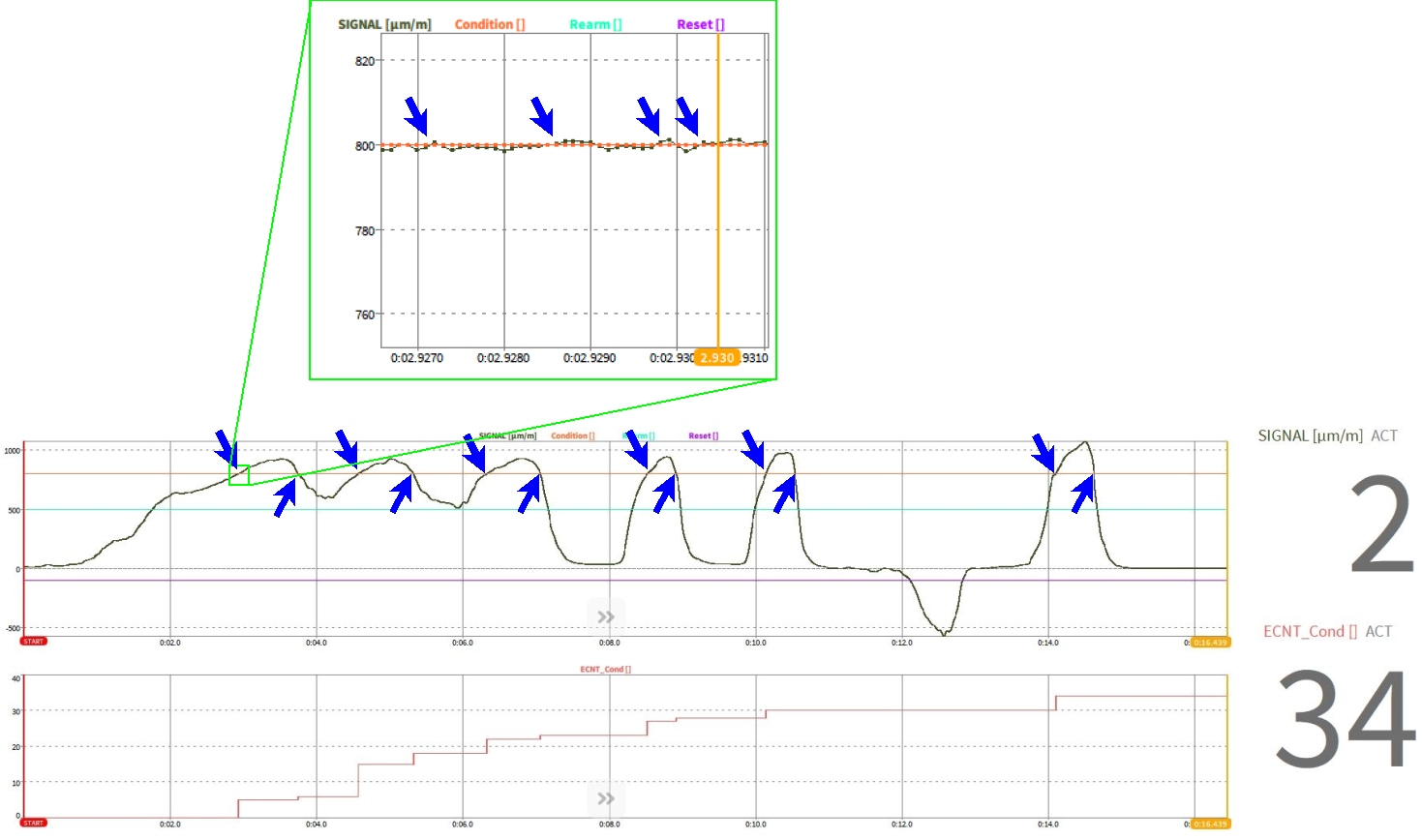
Fig. 229 ECNT-function with Condition only
ECNT_Cond_Rearm = ecnt(‘SIGNAL’>800,’SIGNAL’<500)
If the channel SIGNAL passes 800 with a Rising Edge (>), the channel ECNT_Cond_Rearm increases by 1. To avoid unwanted increments caused by noise on the signal, the channel SIGNAL must pass 500 with a Falling Edge (<) before the channel ECNT_Cond_Rearm counts again when the channel SIGNAL passes 800 with a Rising Edge (>) (see Fig. 230).
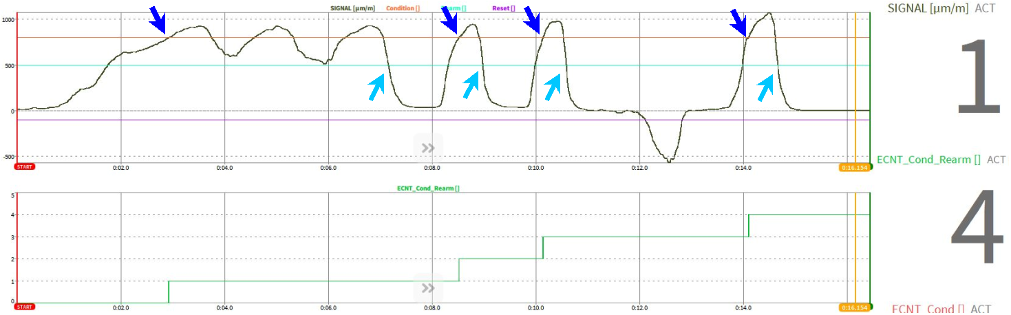
Fig. 230 ECNT-function with Condition and Rearm
ECNT_Cond_Rearm_Reset = ecnt(‘SIGNAL’>800,’SIGNAL’<500,’SIGNAL’<-100)
If the channel SIGNAL passes 800 with a Rising Edge (>), the channel ECNT_Cond_Rearm_Reset increases by 1. To avoid unwanted increments caused by noise on the signal, the channel SIGNAL must pass 500 with a Falling Edge (<) before the channel ECNT_Cond_Rearm_Reset counts again when the channel SIGNAL passes 800 with a Rising Edge (>). If the Channel SIGNAL passes -100 with a Falling Edge (<), the channel ECNT_Cond_Rearm_Reset is set to 0 (see Fig. 231).
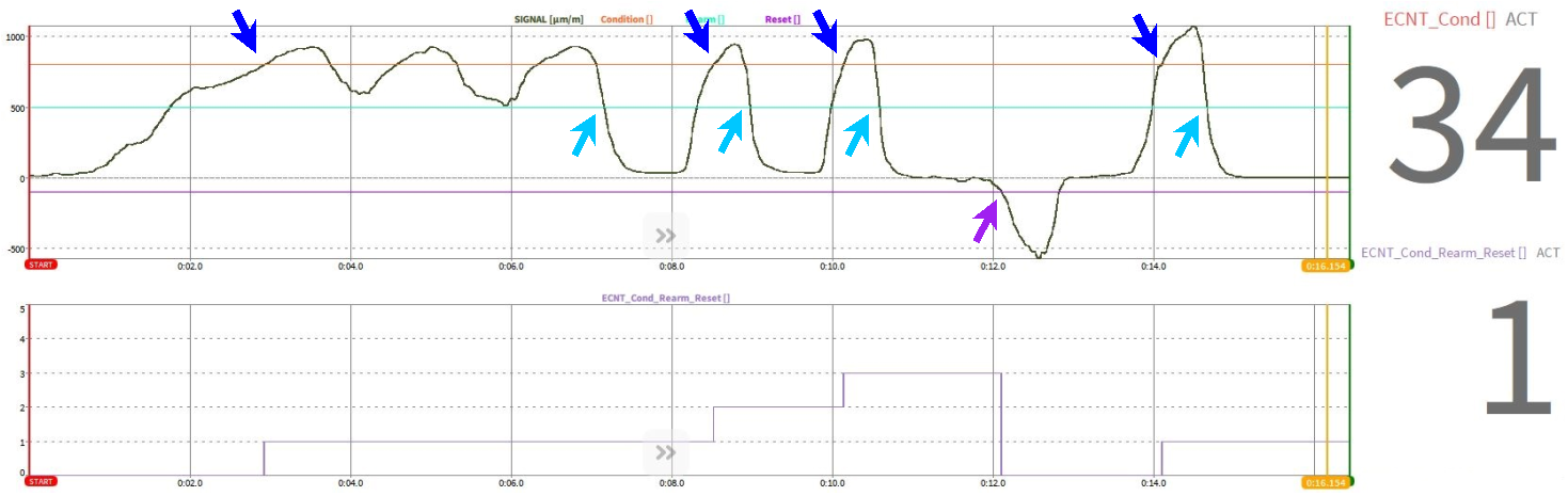
Fig. 231 ECNT-function with Condition, Rearm and Reset
Hold function (hold)
Syntax: hold(value,cond,init,rearm)
The hold-function requires two input channels. One channel is the Signal channel and one channel the Condition channel. If the Condition channel fulfills a certain Condition, the actual value of the Signal channel is stored to the hold-function channel. If desired, an Initial value and a Rearm event which must be passed before a Condition can be fulfilled again, can be defined. Condition and Rearm can be applied to Rising and Falling signal edges. Rising Edges can be defined by using the logical operators > and ≥. Falling Edges can be defined by using the logical operators < and ≤.
The following examples will explain the functionality (corresponding dmd-file can be found here: https://ccc.dewetron.com/pl/OXYGEN):
HOLD_VAL_COND = hold(‘SIGNAL_VAL’,’SIGNAL_COND’>5)
If the channel SIGNAL_COND passes 5 with a Rising Edge (>), the actual value of the channel SIGNAL_VAL is stored to the channel HOLD_VAL_COND. The value of the channel HOLD_VAL_COND is NaN before reaching the Condition the first time (see Fig. 232).
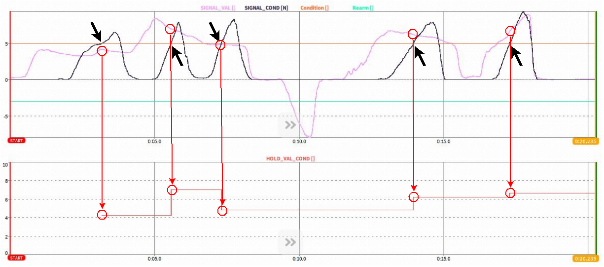
Fig. 232 HOLD function with Condition
HOLD_VAL_COND_INIT = hold(‘SIGNAL_VAL’,’SIGNAL_COND’>5,2)
If the channel SIGNAL_COND passes 5 with a Rising Edge (>), the actual value of the channel SIGNAL_VAL is stored to the channel HOLD_VAL_COND_INIT. The Initial value of the channel HOLD_VAL_COND_INIT is 2 before reaching the Condition the first time (see Fig. 233).
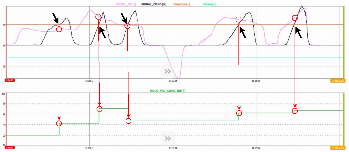
Fig. 233 HOLD function with Condition and Initial value
HOLD_VAL_COND_INIT_REARM = hold(‘SIGNAL_VAL’,’SIGNAL_COND’>5,2,’SIGNAL_VAL’>-3)
If the channel SIGNAL_COND passes 5 with a Rising Edge (>), the actual value of the channel SIGNAL_VAL is stored to the channel HOLD_VAL_COND_INIT_REARM. The Initial value of the channel HOLD_VAL_COND_INIT_REARM is 2 before reaching the Condition the first time. In addition, the channel SIGNAL_VAL must pass -3 with a Rising Edge (>) before the channel HOLD_VAL_COND_INIT_REARM updates again when the channel SIGNAL_COND passes 5 with a Rising Edge (>) (see Fig. 234).
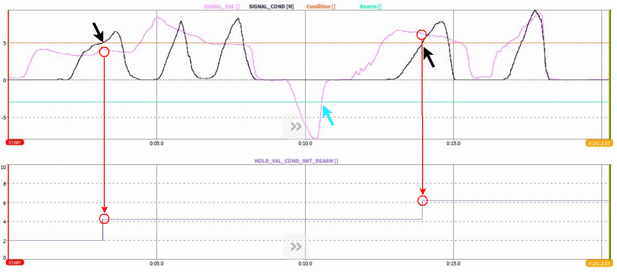
Fig. 234 HOLD function with Condition, Initial value and Rearm level
Stopwatch function (stopwatch)
Syntax: stopwatch(start_cond,stop_cond, reset)

Fig. 235 Schematic explanation of the stopwatch function
The stopwatch function returns the timespan in seconds between two conditions (start_cond and stop_cond). Both conditions may refer to the same channel or to different channels. An optional reset condition resets the stopwatch function to NaN until the next start_cond occurs.
If the reset is not specified, the stopwatch-function restarts to count at 0s automatically at every new start_cond.
If the reset is specified as 0 (i.e. stopwatch (start_cond,stop_cond,0)), the stopwatch function does not restart to count at 0s when a new start_cond occurs but continues counting from the last value.
If the reset is specified differently, i.e. as signal<0, the stopwatch function is reset to NaN if this certain event occurs and starts counting from 0s if a new start_cond occurs.
If the start_cond appears again before a stop_cond is reached, the start_cond will be ignored.
If start_cond is equal to the stop_cond, the stopwatch returns 0s.
The following examples will clarify the functionality of the stopwatch function (corresponding dmd-file can be found here: https://ccc.dewetron.com/pl/OXYGEN):
STOPWATCH_cond1_cond2 = stopwatch(‘SIGNAL1’>100,’SIGNAL1’>800)
The stopwatch function (dark blue graph in Fig. 236) will start to measure the time in seconds if the channel SIGNAL1 (light blue graph in Fig. 236) exceeds 100 and stop to measure the time in seconds if the channel SIGNAL1 exceeds 800. If SIGNAL1 will exceed 100 again, the stopwatch function restarts to measure at 0s.
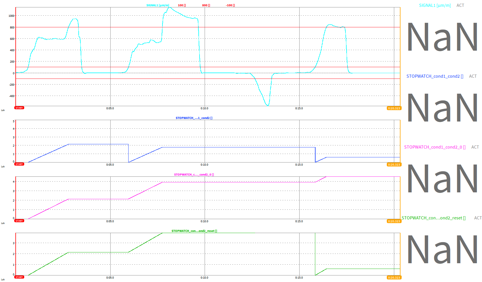
Fig. 236 Stopwatch with start and stop condition
STOPWATCH_cond1_cond2_0 = stopwatch(‘SIGNAL1’>100,’SIGNAL1’>800,0)
The stopwatch function (pink graph in Fig. 237) will start to measure the time in seconds if the channel SIGNAL1 (light blue graph in Fig. 237) exceeds 100 and stop to measure the time in seconds when the channel SIGNAL1 exceeds 800. If SIGNAL1 will exceed 100 again, the stopwatch function restarts to measure from the last value and NOT reset.
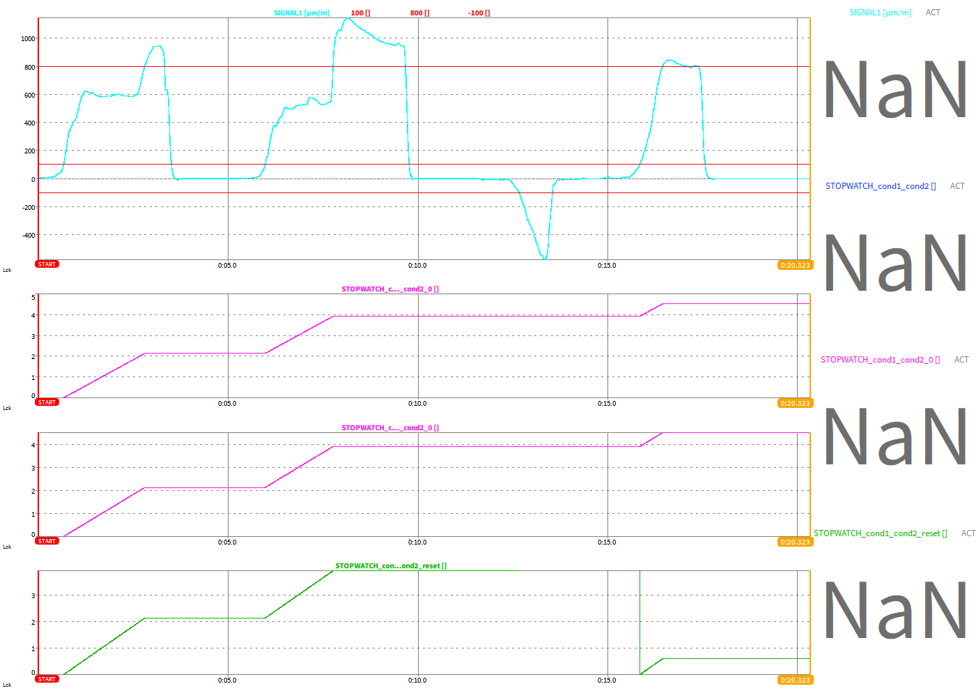
Fig. 237 Stopwatch with start and stop condition, no reset
STOPWATCH_cond1_cond2_reset = stopwatch(‘SIGNAL1’>100,’SIGNAL1’>800,’SIGNAL1’<-100)
The stopwatch function (green graph in Fig. 238) will start to measure the time in seconds if the channel SIGNAL1 (light blue graph in Fig. 238) exceeds 100 and stop to measure the time in seconds when the channel SIGNAL1 exceeds 800. If (and only if) SIGNAL1 decreases below -100, the stopwatch function will reset to NaN and restart to measure from 0s if SIGNAL1 exceeds 100 again.
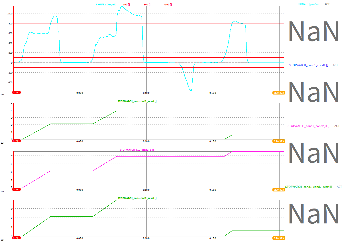
Fig. 238 Stopwatch with start and stop condition, reset specified
Measdiff function (measdiff)
Syntax: measdiff(val,cond1,cond2)
The measdiff function returns the value difference between cond1 and cond2 of the signal val. The three parameters may refer to same channel or each to a different channel.
The measdiff function will return NaN before cond2 is reached for the first time.
If cond1 and cond2 are triggered several times during one measurement, the measdiff function will be updated after cond2 is reached again.
If cond1 is reached several times before cond2 is reached, the measurement will start when cond1 is reached for the first time and will not be reset if cond1 is reached again.
The following examples will clarify the functionality of the measdiff function (corresponding dmd-file can be found here: https://ccc.dewetron.com/pl/OXYGEN):
MEASDIFF_val_cond1_cond2 = measdiff(‘SIGNAL2’,’SIGNAL1’>100,’SIGNAL1’>800)
The measdiff function (purple graph in Fig. 239) will measure and return the value difference of SIGNAL2 (green graph in Fig. 239) triggered by the following conditions: The measurement is initialized when SIGNAL1 (light blue graph in Fig. 239) exceeds 100 and stopped when SIGNAL1 exceeds 800.
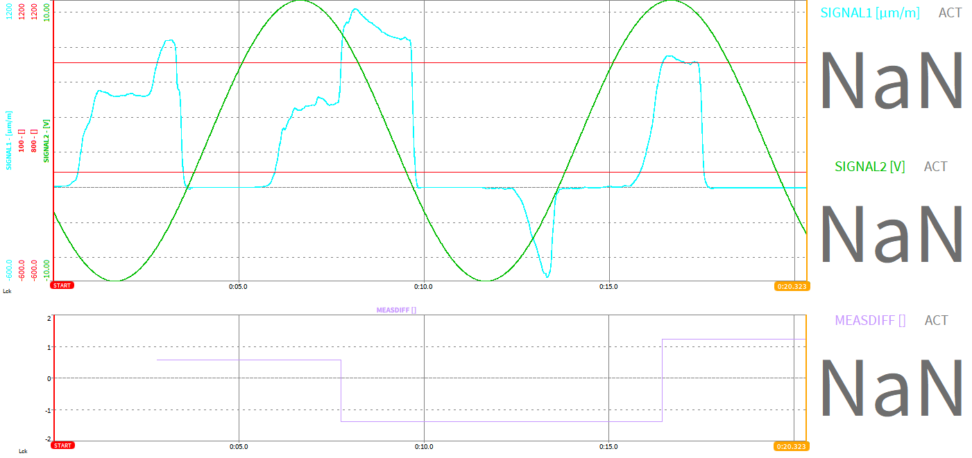
Fig. 239 Measdiff function
Period function (period)
Syntax: period(cond,[rearm])
The period function returns the period time of a signal in seconds. The signal to which the function shall be applied to must be specified in the cond in combination with the period threshold which is normally zero.
An optional rearm level will suppress distortion caused by signal noise. The rearm can be applied to the same or to a different signal.
The following examples will clarify the functionality of the period function (corresponding dmd-file can be found here: https://ccc.dewetron.com/pl/OXYGEN):
PERIOD_cond = period(‘SIGNAL’>0)
The period function (green graph in Fig. 240) will measure and return the period time of SIGNAL (brown graph in Fig. 240) for the condition that the SIGNAL level is higher than 0. As the SIGNAL is a pure sine wave with frequency 0.5 Hz, its period time should be 2 seconds. But due to noise on the signal, the zero-level is crossed several times (see Fig. 241) and causes a wrong measurement result when determining the period time. To suppress the influence of noise on the period time determination, a rearm level can be optionally added. This is explained in the next section.
PERIOD_cond_rearm = period(‘SIGNAL’>0,’SIGNAL’>-5)
The period function (green graph in Fig. 240) will measure and return the period time of SIGNAL (brown graph in Fig. 240) for the condition that the SIGNAL level is higher than 0. As period time measurements can be disturbed by noise, a rearm level is added in this example to avoid the influence of noise to the signal. The rearm level is set to the following condition: The level of the SIGNAL must exceed -5. This means that the SIGNAL must exceed -5 before the condition SIGNAL>0 is detected again. With this optional rearm level the influence of noise on the period time measurement that can be seen in the green graph of Fig. 240 is suppressed and the detected period time is always 2s as it can be seen in the blue graph of Fig. 240.
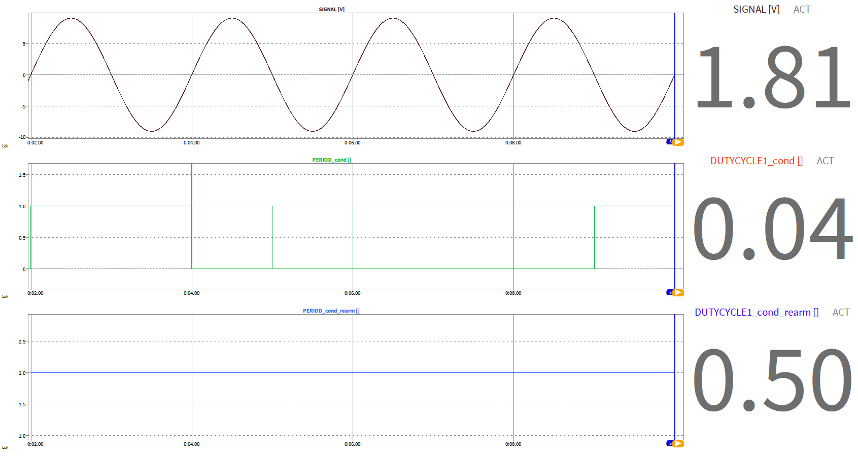
Fig. 240 Period function
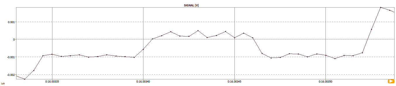
Fig. 241 Noise disturbing the correct functionality of the period determination
Dutycycle function (dutycylce)
Syntax: dutycylce(cond,[rearm])
The dutycycle function returns the dutycycle of a signal. The signal to which the function shall be applied to must be specified in the cond in combination with the dutycylce threshold.
An optional rearm level will suppress distortion caused by signal noise. The rearm can be applied to the same or to a different signal.
The following examples will clarify the functionality of the dutycycle function (corresponding dmd-file can be found here: https://ccc.dewetron.com/pl/OXYGEN):
DUTYCYCLE_cond = dutycycle(‘SIGNAL’>0)
The dutycylce function (orange graph in Fig. 242) will measure and return the dutycycle of SIGNAL (brown graph in Fig. 242) for the condition that the SIGNAL level is higher than 0. As the SIGNAL is a pure sine wave, its duty cycle should be 0.5 (or 50%). But due to noise on the signal, the zero-level is crossed several times (see Fig. 243) and causes a wrong measurement result when determining the dutycycle. To suppress the influence of noise on the dutycycle determination, a rearm level can be optionally added. This is explained in the next section.
DUTYCYCLE_cond_rearm = dutycycle(‘SIGNAL’>0,’SIGNAL’>-5)
The dutycylce function (orange graph in Fig. 242) will measure and return the dutycycle of SIGNAL for the condition that the SIGNAL level is higher than 0. As dutycycle measurements can be disturbed by noise, a rearm level is added in this example to avoid the influence of noise to the signal. The rearm level is set to the following condition: The level of the SIGNAL must exceed -5. This means that the SIGNAL must exceed -5 before the condition SIGNAL >0 is detected again. With this optional rearm level the influence of noise on the dutycylce measurement that can be seen in the orange graph of Fig. 243 is suppressed and the detected dutycycle is always 0.5 (50%) as it can be seen in the blue graph of Fig. 243.
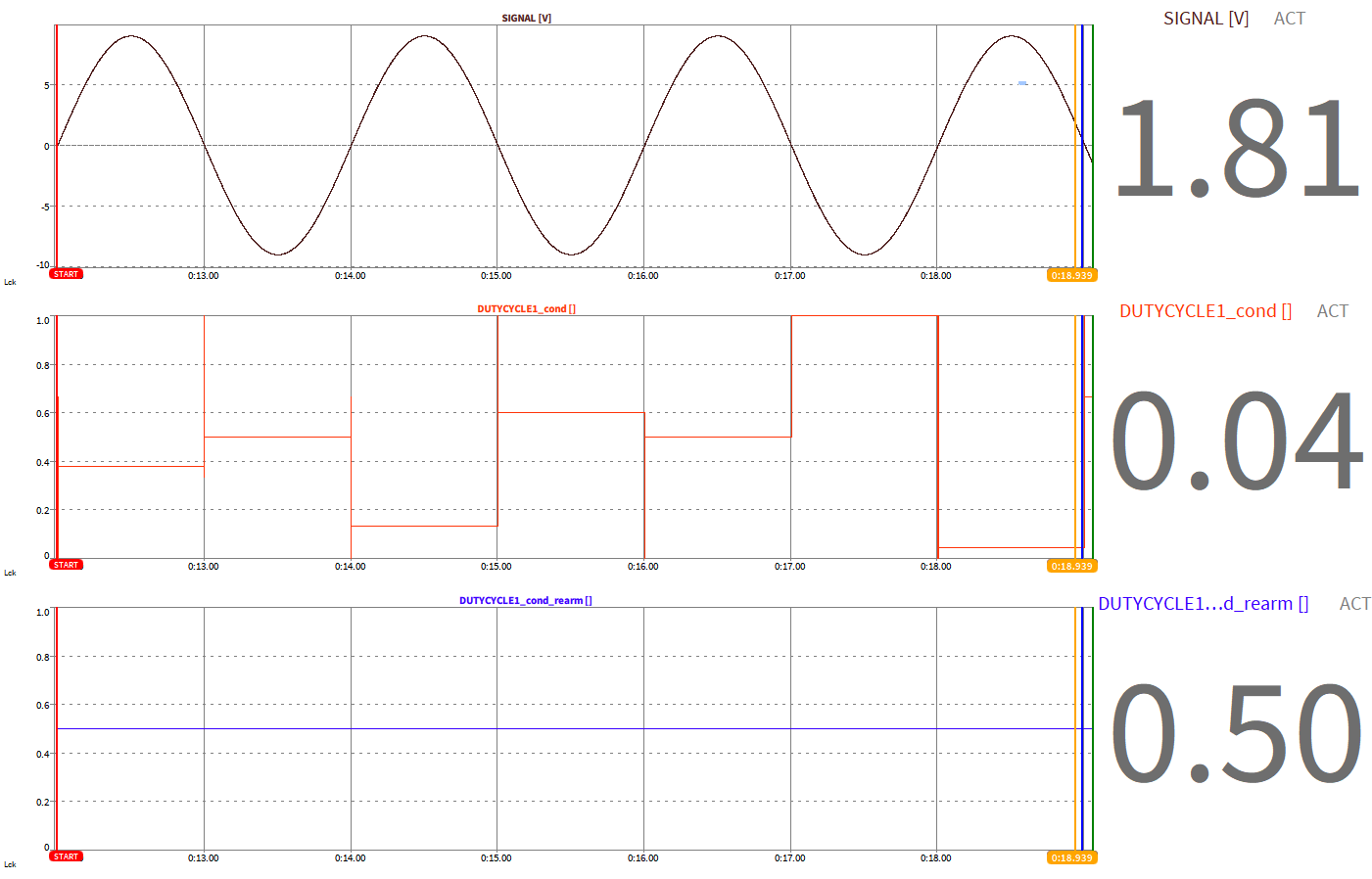
Fig. 242 Dutycycle function
Fig. 243 Noise disturbing the correct functionality of the dutycycle determination
Edge function (edge)
Syntax: edge(cond,rearm)
The edge function returns a rising egde from 0 to 1 in case the condition is passed and a falling edge from 1 to 0 if the rearm is passed.
The following examples will clarify the functionality of the edge function (corresponding dmd-file can be found here: https://ccc.dewetron.com/pl/OXYGEN):
EDGE_cond_ream = edge(‘SIGNAL’>800, ‘SIGNAL’<-100)
The edge function (green graph in Fig. 244) will return a rising edge from 0 to 1for the condition that the SIGNAL level exceeds 800 (brown graph in Fig. 244). In case the SIGNAL falls below -100, the edge function will return a falling edge from 1 to 0.
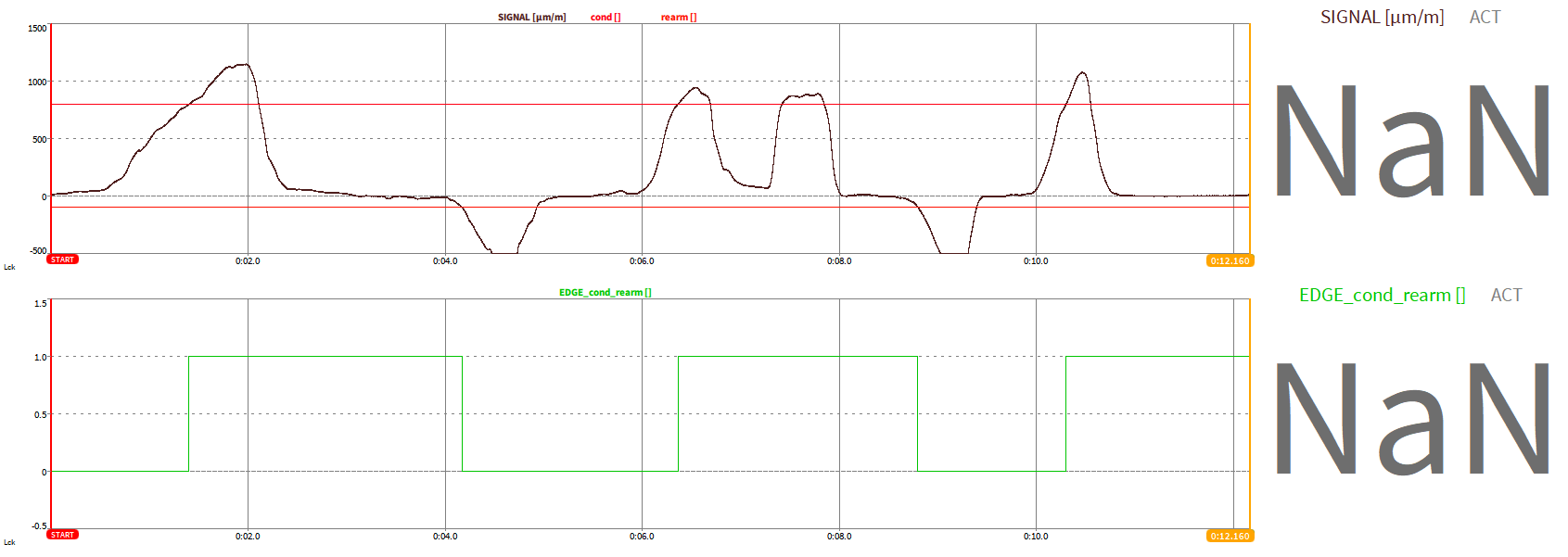
Fig. 244 Edge function
Combination of edge function and other formulas
In case a formula that does not contain a rearm level as optional parameter, such as the stopwatch function (see Stopwatch function (stopwatch)) or the measdiff function (see Measdiff function (measdiff)), the edge function (see Edge function (edge)) can be used to generate this rearm level.
The following example will clarify the functionality by demonstration the combination of the edge and stopwatch function (corresponding dmd-file can be found here: https://ccc.dewetron.com/pl/OXYGEN):
The blue signal in Fig. 245 will measure the time using the stopwatch between the following two conditions: cond1 is true if SIGNAL1 (green signal in Fig. 245) exceeds 100. Cond2 is true if SIGNAL1 (green signal in Fig. 245) exceeds 800.
The formula syntax of the blue signal in Fig. 242 is the following:
stopwatch(‘SIGNAL1’>100,’SIGNAL1’>800)
Due to noise, cond1 is passed several times which might be undesired. To suppress this influence of noise a rearm level of -100 can be added for cond1 by using the edge function. The result can be seen in the orange graph of Fig. 245. In this example, the stopwatch function is only restarted if SIGNAL1 falls below -100.
The syntax is the following:
stopwatch(edge(‘SIGNAL1’>100,’SIGNAL1’<-100)>0.5,’SIGNAL1’>800)
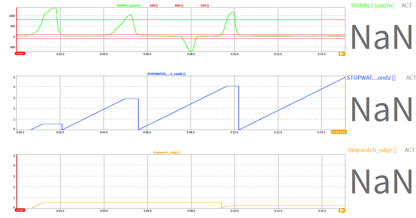
Fig. 245 Combination of edge and stopwatch function
Rolling-overall-functions
rmin(value[,reset])
Returns the global minimum of the signal specified as value from acquisition start until the current instant of time; Is reset at measurement start; Can be optionally reset by specifying a reset condition; The update rate is equal to the sample rate of the channel with the highest sample rate that is assigned to this formula.
rmax(value[,reset])
Returns the global maximum of the signal specified as value from acquisition start until the current instant of time; Is reset at measurement start; Can be optionally reset by specifying a reset condition; The update rate is equal to the sample rate of the channel with the highest sample rate that is assigned to this formula.
ravg(value[,reset])
Returns the global arithmetic average of the signal specified as value from acquisition start until the current instant of time; Is reset at measurement start; Can be optionally reset by specifying a reset condition; The update rate is equal to the sample rate of the channel with the highest sample rate that is assigned to this formula.
rrms(value[,reset])
Returns the global RMS of the signal specified as value from acquisition start until the current instant of time; Is reset at measurement start; Can be optionally reset by specifying a reset condition; The update rate is equal to the sample rate of the channel with the highest sample rate that is assigned to this formula.
rsum(value[,reset])
Returns the global sum of the signal specified as value from acquisition start until the current instant of time; Is reset at measurement start; Can be optionally reset by specifying a reset condition; The update rate is equal to the sample rate of the channel with the highest sample rate that is assigned to this formula.
racrms(value[,reset])
Returns the global ACRMS of the signal specified as value from acquisition start until the current instant of time; Is reset at measurement start; Can be optionally reset by specifying a reset condition; The update rate is equal to the sample rate of the channel with the highest sample rate that is assigned to this formula.
For details about the ACRMS, refer to Statistics channel.
rp2p(value[,reset])
Returns the global peak-to-peak level of the signal specified as value from acquisition start until the current instant of time; Is reset at measurement start; Can be optionally reset by specifying a reset condition; The update rate is equal to the sample rate of the channel with the highest sample rate that is assigned to this formula.
A corresponding dmd-file can be found here: https://ccc.dewetron.com/pl/OXYGEN
Array channels in formulas
Array channels in OXYGEN are data channels (or vectors) that include several data elements for one instance of time, such as harmonics from a powergroup, amplitude spectra of a FFT calculation or a CPB spectrum. Using OXYGEN, Array channels are typically either visualized by using an Array Chart or a Spectrum Analyzer.
Besides time based synchronous and asynchronous channels it is also possible work with array channels in the Formula editor.
Mathematical operations with array channels
The following mathematical operations are supported when using array channels in formulas:
Basic math operations for arrays with same dimensions supported (see ① in Fig. 246): + - * /
Operations (+ - * /) with arrays and constants (see ② in Fig. 246)
In both cases, the output of the formula will be a new array channel.
Fig. 246 Basic math operations for arrays
In addition to that, it is possible to use the following operators in combination with array channels:
Standard operators (see Fig. 247)
Fig. 247 Standard operators in combination with array channels
Trigonometric operators (see Fig. 248)
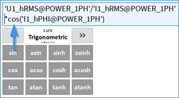
Fig. 248 Trigonometric operators in combination with array channels
Logic operators (see Fig. 249)
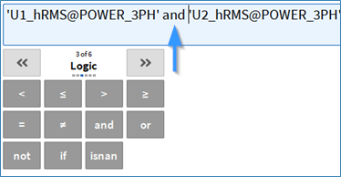
Fig. 249 Logic operators in combination with array channels
The formula output will be a new array channel here as well.
Extraction of array elements
It is possible to extract one or several elements from an array channel into a new array channel. The syntax for that is following the Python programming language:
The first element of an array has always the index 0.
When extracting several adjacent elements, the first specified index is always inclusive and the last one is always exclusive (see Fig. 251)
The following options for extracting array elements exist:
Extraction of one dedicated element (see Fig. 250). The output will be an asynchronous time domain channel
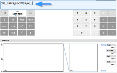
Fig. 250 Extraction of one dedicated element
Extraction of several adjacent elements (see Fig. 251). The output will be an array channel with the number of extracted element as new dimension.
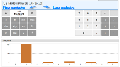
Fig. 251 Extraction of several adjacent elements
Extraction of several adjacent elements with a step size between the elements to be extracted (see Fig. 252). The output will be an array channel with the number of extracted element as new dimension.
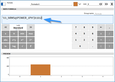
Fig. 252 Extraction of several adjacent elements with step size between the elements to be extracted
Creation of arrays with constants
Finally, it is possible to create array channels with constant elements (see Fig. 253). The update rate can be defined by adding a time domain channel and multiplying it with zero. The array will then have the same update rate as the time domain channel.
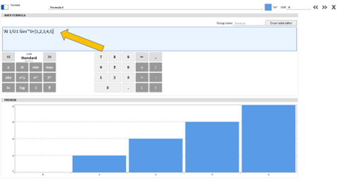
Fig. 253 Creation of arrays with constant elements
Statistics channel
To create Statistic channels, click on the [+] button in the lower-left corner of the Data Channels menu (see Working with Software Channels) and select Statistics. Before doing so, you must select the input channel(s). Multiple input channels can be selected to create multiple Statistics channels with identical settings.
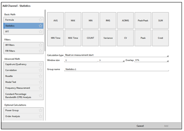
Fig. 254 Pop-up window for creating a statistics channel
In the Add Channel pop-up, you can select which statistical parameter should be calculated. For each parameter, OXYGEN will create an individual output channel. Further, general configurations include:
Calculation Type – multiple types are available, see below for a detailed description.
Windows size – define the size of the calculation window
Overlap – define window overlap; see Fig. 257.
Group name – define group name to organize channels in Data Channels menu.
The defined channel parameters can be changed afterwards in the Channel Setup (see Fig. 258).
Available statistical parameters
i = 1…N
N = Sample Rate of Input Channel * Window Size
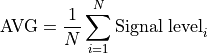
AVG: Calculates the linear mean value for the selected Window size according to the following formula:
MAX: Calculates the maximum signal level appearing in the individual time window

MIN: Calculates the minimum signal level appearing in the individual time window

RMS: Calculates the quadratic mean value (RMS) for the selected window size according to the following formula
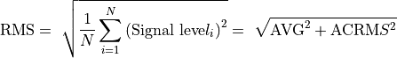
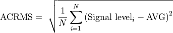
ACRMS: Calculates the quadratic mean value which is revised from DC components. This value is identical to the standard deviation calculated according to the following formula
Peak-Peak: Calculates the peak-peak value for the selected window size by following formula:

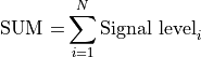
SUM: calculates the sum of the signal level within the window size by following formula
MIN Time: Determines the time, where the minimum of the signal was reached.
MAX Time: Determines the time, where the maximum of the signal was reached.
COUNT: Counts the number of samples within a calculation window.
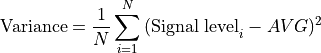
Variance: Calculates the variance, which is calculated by the squared ACRMS value by following formula:
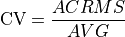
CV: Calculates the coefficient of variation by following formula
Peak: Calculates the peak value by following formula

Crest: Calculates the crest factor by following formula
Frequency: Calculates the frequency of Start trigger level events and averages over N periods. This is only available for the Phase-Locked calculation type and one selected channel.

Period Time: Measures the time between Start trigger level events and averages over N periods. This is only available for the Phase-Locked calculation type and one selected channel.

Note
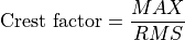
Difference between the RMS and the ACRMS value: The RMS and the ACRMS value of a signal without DC component is the same. Let’s assume a sine wave with an amplitude of 1 and no DC offset:
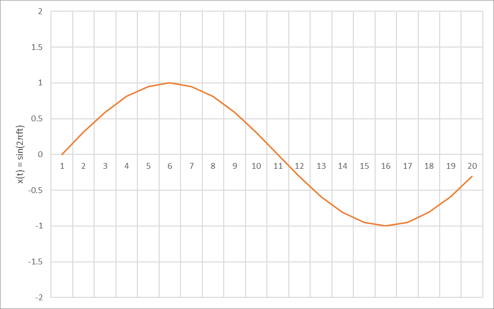
Fig. 255 Sine wave with amplitude 1, no DC component
In this case the RMS value is ~0.707 and the ACRMS value is ~0.707 as well.
If the signal has a DC component, the RMS value respects this DC component, but the ACRMS value does not respect the DC component:
Fig. 256 Sine wave with amplitude 1, 0.5 DC component
For this signal, the RMS value is ~0.866, because the DC component is respected, but the ACRMS value is again ~0.707, because the DC component is not respected.
Available calculation types
Reset on measurement start
In this mode, the statistic resets at the start of each measurement. The calculation uses a defined window size and an optional overlap.
Continuous
The statistic is calculated continuously without resetting at the beginning of a measurement. Like Reset on measurement tart, it also requires a window size and optionally an overlap.
Overall
This mode produces a single statistical value based on all acquired data points over the entire recording. In a recorder instrument, this appears as a horizontal line. No additional parameters are required.
Triggered
The calculation starts only when a trigger event occurs. This mode allows highly controlled, event-based evaluations. You can define the trigger channel, trigger level, whether the trigger reacts to a rising or falling edge, a rearm level and the stop mode. For stop mode you can either choose: Stop Trigger – calculation stops based on another trigger event, Duration – calculation length is defined via time interval, Retrigger – start-trigger configuration is also used as the stop condition.
Running
The statistic updates at the same rate as the input channel. For every new incoming sample, the calculation looks back over a defined window size and computes the statistic for that time window. Since the window typically contains many samples, this mode provides a constantly updated moving statistic.
Phase-Locked
Statistics of the reference channel are synchronized to the period source channel. By default the period source channel is the same as the first selected channel. The statistics time window can be set for N periods (1 to 1000). The periods are detected based on the trigger level of the period source channel. The Phase-Locked mode has two additional statistic types, Frequency and Period time. These are calculated based on the periods source chanel for every period and averaged over N periods.
Window overlapping
The following figure shows the mechanism for the statistics calculations and how the calculation window is moved.
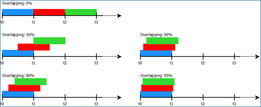
Fig. 257 Overlapping mechanism for the statistic calculations
Channel setup overview
Fig. 258 and Table 24 provide an overview of channel setup for statistical channels using the example of RMS statistics.
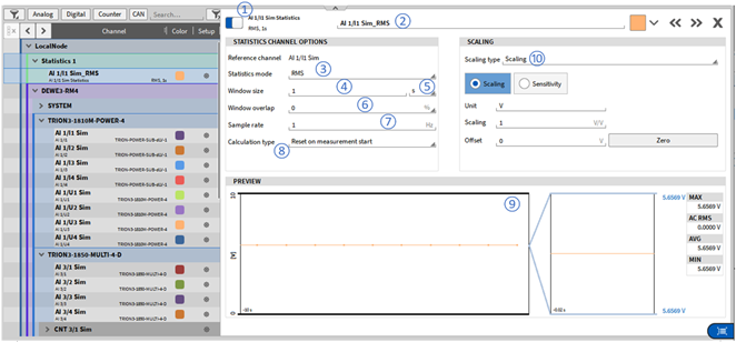
Fig. 258 Statistics Channel Setup Overview
No. |
Function |
Description |
|---|---|---|
1 |
Active button |
Setting a channel active or inactive; An active channel can be displayed in an instrument, used in a math channel and can be recorded, an inactive channel not. |
2 |
Channel name |
Individual channel name; Can be changed individually. |
3 |
Group name |
Change the name of the statistics grouping. |
4 |
Statistics Mode |
Select the statistical value that shall be calculated. |
5 |
Calculation type |
Select if the calculation should be carried on continuously, if the calculation should be reset on measurement start or if an overall value (single value) over the recording duration should be calculated. |
6 |
Window Size |
Type in the desired window size (will affect the Sample Rate ⑥). |
7 |
Window Size Unit |
Select the unit of the window size. Select between seconds (s), minutes (m), hours (h) and days (d) (will affect the Sample Rate ⑥). |
8 |
Window overlap |
Choose a window overlap between 0 and 99 %. |
9 |
Sample Rate |
Sample rate that is calculated from the Window size in Hz (Window Size can also be changed via Sample Rate changes). |
10 |
Scaling menu |
Change the channels’ scaling by entering a Scaling factor or changing the sensitivity (and/or entering an offset) or by a 2-point scaling. |
Using Array channels in Statistics
Besides time-based synchronous and asynchronous channels, it is also possible to assign array channels to Statistics calculations. The calculation is created in the same manner as for time domain channel. The resulting statistic channel will be another array with same dimensions as the source channel. The update rate will be equal to the statistics window size. This means the statistical analysis is done on a bin-by-bin basis.
For a description of the difference between “Using Array channels in Statistics” and “Array Statistics” see Difference between Array Statistics and Statistics calculated for array channels.
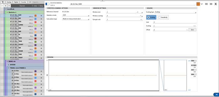
Fig. 259 Resulting statistics channels based on an array channel
FFT channels
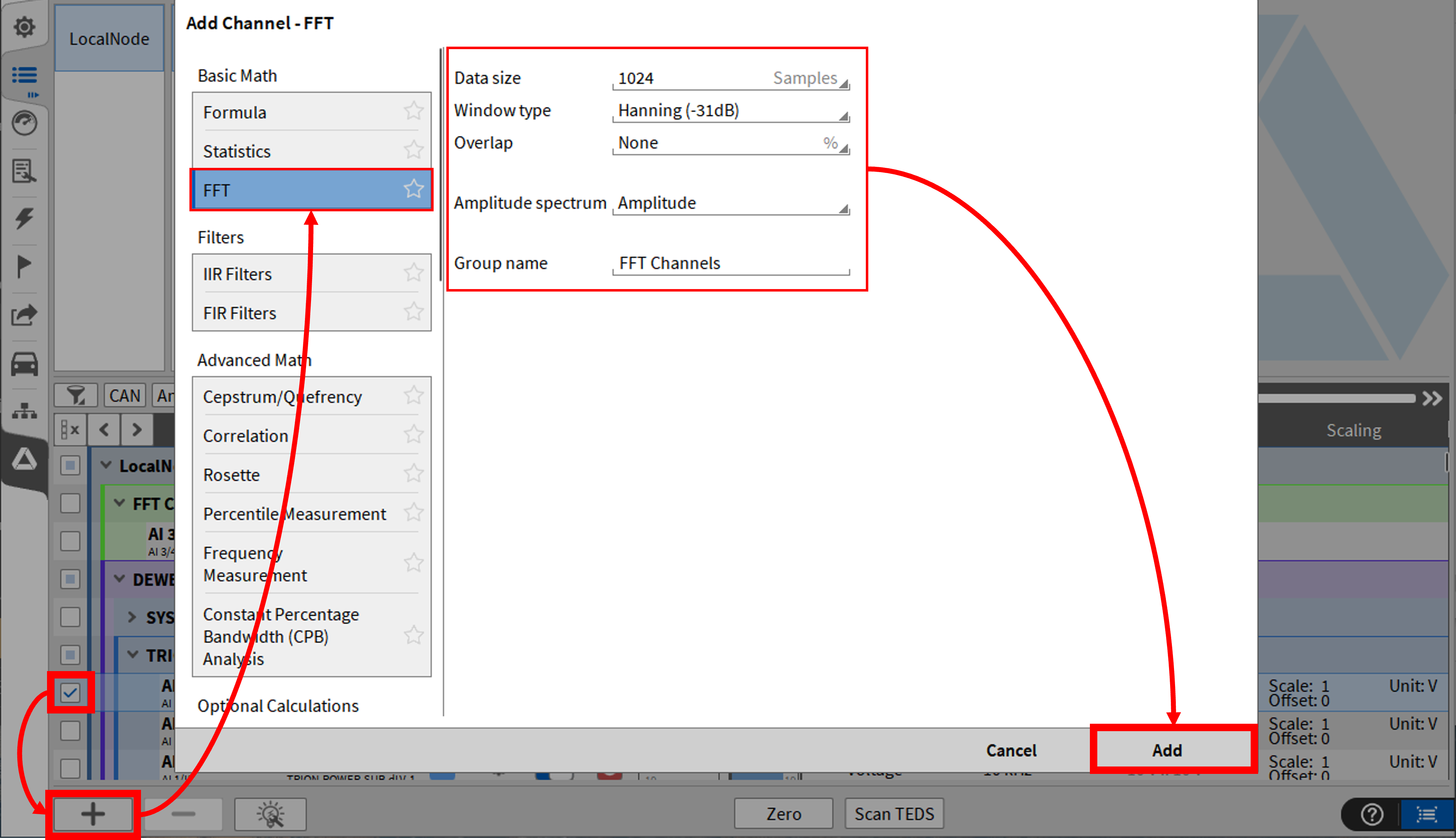
Fig. 260 Pop-up window for creating an FFT channel
For creating a FFT channel, the user must select the channel and then click on the Add button in the lower left corner (marked red in Fig. 224) and select FFT in the appearing window (see Fig. 266). The user can select several input channels simultaneously to create several FFT channels with the same settings at once.
Note
FFT math can only be applied to synchronous channels, such as analog input channels or counter channels but not to asynchronous channels, CAN channels, EPAD cannels, or power group channels.
Note
The difference between the FFT calculation using this math module or the Instrument Spectrum Analyzer is that the calculation using the math module is deterministic and the calculation using the Spectrum Analyzer is stochastic, i.e. the deterministic calculation can always be reproduced, because the exact instant of time each FFT spectrum is calculated is contained. This is not the case for stochastic calculation.
In addition, as the FFT calculation using the math module results in own FFT channels, the data can be exported to third party formats using the Export menu in the PLAY mode (for details, refer to Export Settings). This is not the case for the calculation using the Spectrum Analyzer.
Five channels may be created for each FFT calculation:
The channel containing the complex spectrum Yk (called Channel_Name_Cpx). This channel cannot be visualized with an OXYGEN Instrument but is only useful for exporting it and using it for post-processing in a 3rd party software.
The channel containing the amplitude spectrum Ak (called Channel_Name_Amp) which is calculated according to the following formula:


This channel can be visualized within OXYGEN using the Spectrum Analyzer (see Spectrum analyzer) if the actual spectrum shall be plotted or it may also be assigned to the Spectrogram Instrument (see Spectrogram) if the time dependent spectral trend shall be displayed.
The channel containing the phase spectrum φk (called Channel_Name_Phi) which is calculated according to the following formula:
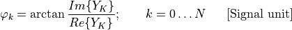
This channel can be visualized within OXYGEN using the Spectrum Analyzer (see Spectrum analyzer) if the actual spectrum shall be plotted or it may also be assigned to the Spectrogram Instrument (see Spectrogram) if the time dependent spectral trend shall be displayed.
This channel is not calculated automatically but must be selected manually in the Channel Setup of the complex spectrum Channel Channel_Name_Cpx after creating the FFT channel (see ⑭ in Fig. 262).
The channel containing the overall peaks of the amplitude spectrum
This channel is deactivated by default and holds the maximum of the amplitude values for each bin over the acquisition time.
The channel containing the overall average of the amplitude spectrum
This channel is deactivated by default and holds the average of the amplitude values for each bin over the acquisition time.
The channel containing the overall exponential average of the amplitude spectrum
This channel is deactivated by default and holds the exponential average of the amplitude values for each bin over the acquisition time. For detailed description of this method see Table 25.
After selecting the FFT section, the user can define the following FFT characteristics:
Data size: Select the number of samples to be transformed simultaneously into the frequency domain here. The data size may vary between 42 to 16777216 (224) samples. For calculation details, refer to FFT properties for Time Domain Channels.
Window Type: Select an appropriate Window function here. The following windows are available: Hanning, Hamming, Rectangular, Blackman, Blackman-Harris, Flat Top or Bartlett. For calculation details, refer to Window type.
Frequency weighting: If no frequency weighting is required, Z (none) is set as default. Additionally, A, B, C and D weighting are available.
Overlap: Select an overlapping factor from 0 to 99.97559 % here. For calculation details, refer to Calculation of the Periodogram - Averaging of FFT windows.
Amplitude Spectrum: Select the type of amplitude spectrum the Amplitude channel shall con- tain. The following amplitude spectra are available: Amplitude, Amplitude_RMS, Amplitude2, PSD, PSD TISA, PSD MSA, PSD SSA, Decibel (Ref:1), Decibel_RMS (Ref:1), Decibel_Max_Peak (Ref: Max), Decibel V-RMS, Decibel U-RMS, Sound Pressure Level or Sound Pressure Level (Water). For calculation details, refer to Section Spectrum.
If None is selected, no amplitude spectrum channel Channel_Name_Amp but only the complex spectrum channel is created.
Group Name: Define a group in the Channel List to which the channel shall be added
Bin reduction: Reduces the calculated FFT array for all FFT channels to a certain number of spectral lines in relation to the line resolution.
After pressing the Add button, the FFT for the selected input channel(s) will be calculated and the Output channels will be visible within the FFT Channels topology in the Channel List (see Fig. 261).
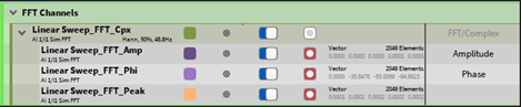
Fig. 261 FFT channels within the channel list
Channel Setup of the Complex spectrum channel
After creating the FFT channel, the following options can be added afterwards within the Channels Setup of the complex Spectrum channel Channel_Name_Cpx:
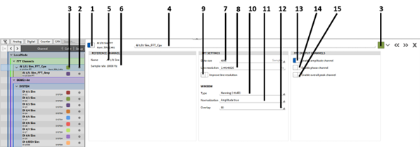
Fig. 262 Complex FFT channel setup - overview
No. |
Function |
Description |
|---|---|---|
1 |
Channel color |
Color scheme of the channel can be changed here. |
2 |
Channel setup |
Open channel settings window |
3 |
Active toggle |
Setting a channel active or inactive; An active channel can be displayed in an instrument, used in a math channel and can be recorded, an inactive channel not |
4 |
Name (of input channel) |
The name of the input channel for the FFT calculation. |
5 |
Sample rate (of input channel) |
The sample rate of the input channel is displayed here. |
6 |
Channel name |
Individual channel name; can be changed individually. |
7 |
Group name |
FFT channels can be grouped. By default, all FFT channels are put into the FFT Channels group. This can be changed at any time. |
8 |
Data size |
Select the number of samples to be transformed to the frequency domain here. The data size can be between 42 to 16777216 (2^24) samples. This automatically results in a certain line resolution. For calculation details, refer to FFT properties for Time Domain Channels. |
9 |
Line resolution selection |
Instead of selecting the number of samples, the line resolution in Hz can be entered, for which the data size is calculated. For calculation details, refer to FFT properties for Time Domain Channels . |
10 |
Improve Line Resolution selection |
Enable Zero-Padding here. For calculation details, refer to Additional information: improve line resolution (Enable zero-padding). |
11 |
Window Type selection |
Select an appropriate Window function here. The following windows are available: Hanning, Hamming, Rectangular, Blackman, Blackman-Harris, Flat Top or Bartlett. For calculation details, refer to Window type. |
12 |
Normalization Type selection |
Select between Amplitude True, Power True or No normalization. For calculation details, refer to Normalization of FFT Spectra. |
13 |
Overlap selection |
Select an overlapping factor from 0 to 99.97559% here. For calculation details, refer to Markers. |
14 |
Enable Amplitude channel selection |
Enable or disable the calculation of the amplitude channel here; enabled per default. |
15 |
Enable Phase channel selection |
Enable or disable the calculation of the phase channel here; disabled per default. |
16 |
Enable Overall Peak channel selection |
Enable or disable the calculation of the total peak channel (see Fig. 262); disabled per default. |
17 |
Enable overall RMS average selection |
Enable or disable the calculation of the total overall RMS average channel (see Fig. 262); disabled per default. |
18 |
Enable overall exponential average selection |
Enable or disable the calculation of the total overall exponential
average channel, with following formula. y*n= α*x(n)+(1-α)*y*(n-1) and α=1-e^(ΔT/ |
19 |
Exponential time constant |
|
20 |
Overall Mode |
Can be set to 3 modes, which affects all overall channels: - Overall (Default): Averaging from measurement start to end - Block based: Averaging multiple spectra for a certain number of spectra - Time based: Averaging multiple spectra for a certain timespan |
21 |
Overall duration |
Only visible when selecting Block based or Time based as Overall Mode. The block size or timespan for the FFT calculation can be set here, depending of the selection of the Overall mode. |
22 |
Minimum frequency |
Selection of the minimum frequency for the FFT calculation from 0 to half of the sampl erate of the base channel. |
23 |
Maximum frequency |
Selection of the maximum frequency for the FFT calculation from Minimum frequency to half of the sample rate of the base channel. |
24 |
Bin reduction |
Reduces the FFT bins to the defined spectral lines, e.g. 1st, 2nd and 5th order in relation to the line resolution. |
 )
)Channel Setup of the Amplitude spectrum channel
After creating the FFT channel the following options can be added afterwards within the Channels Setup of the Amplitude Spectrum channel Channel_Name_Amp:
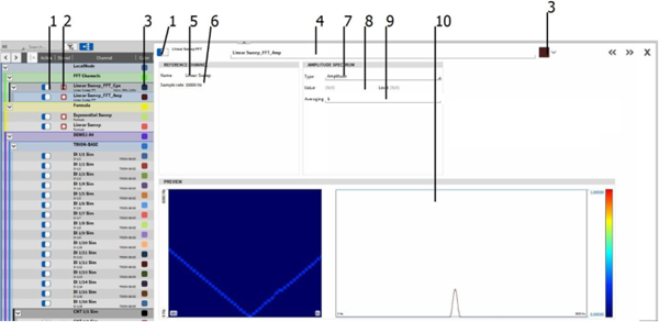
Fig. 263 Amplitude FFT channel setup - overview
No. |
Function |
Description |
|---|---|---|
1 |
Color |
The color scheme of the channel can be changed here. |
2 |
Channel setup |
Open channel settings window |
3 |
Active button |
Setting a channel active or inactive; An active channel can be displayed in an instrument, used in a math channel and can be recorded, an inactive channel not. |
4 |
Name (of input channel) |
The name of the input channel for the FFT calculation. |
5 |
Sample rate (of input channel) |
Sample rate of the input channel is displayed here. |
6 |
Channel name |
Individual channel name; Can be changed individually. |
7 |
Spectrum type selection |
Change the type of the amplitude spectrum here. For calculation details and spectra to be selected, refer to Section Spectrum. |
8 |
Value selection |
If Decibel or Decibel RMS spectrum type is selected, the reference value can be entered here. |
9 |
Frequency weighting |
Select if a frequency weighting should be applied to the amplitude spectrum A, B, C, D or Z (none) are available. |
10 |
Averaging selection |
Average over 1 to 16 spectra. |
11 |
Preview window |
Preview of the calculation in time (left) and frequency domain (right). |
Channel Setup of the Phase spectrum channel
After creating the FFT channel, the following options can be added afterwards within the Channels Setup of the Phase Spectrum channel Channel_Name_Phi:
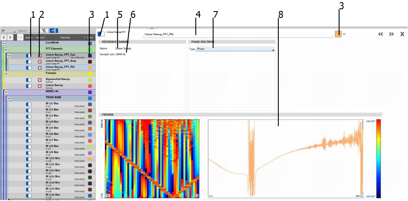
Fig. 264 Phase FFT channel setup - overview
No. |
Function |
Description |
|---|---|---|
1 |
Color |
The color scheme of the channel can be changed here. |
2 |
Channel setup |
Open channel settings window. |
3 |
Active button |
Setting a channel active or inactive; An active channel can be displayed in an instrument, used in a math channel and can be recorded, an inactive channel not. |
4 |
Name (of input channel) |
The name of the input channel for the FFT calculation. |
5 |
Sample rate (of input channel) |
Sample Rate of the input channel is displayed here. |
6 |
Channel name |
Individual channel name; can be changed individually |
7 |
Spectrum type selection |
Change the type of the phase spectrum here. Available types are Phase, Phase unwrapped, Phase (radiant) and Phase unwrapped (radiant). For calculation details and spectra to be selected, refer to Section Spectrum. |
8 |
Preview window |
Preview of the calculation in time (left) and frequency domain (right). |
Channel Setup of Overall Channels
For overall channels, namely the overall peak, overall RMS and overall exponential average channel, no settings can be changed within the Channels Setup after the FFT channels have been created. It is only possible to change the name of the channel and to activate or deactivate them.
All overall channels are based on the amplitude channel of the FFT. If the amplitude channel will be deactivated all overall channels will be deactivated automatically too.
The following figure shows all three amplitude channel types: the amplitude channel, the total peak value, the total RMS average value and the exponential average of the amplitudes.
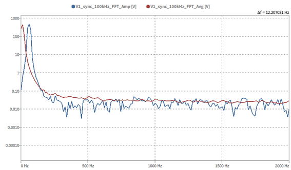
Fig. 265 Example of amplitudes, overall peak, overall RMS average, overall exponential average in the spectral view
Filters
IIR Filter channel
To create IIR filtered channels, click on the [+] button in the lower-left corner of the Data Channels menu (see section Working with Software Channels) and select IIR Filters. Optionally, the filter type, filter frequency, filter characteristic including the order and the filter group name can be defined at the filter creation. These parameters can be changed also after clicking Add. For all selected input channels, a filter channel is created.
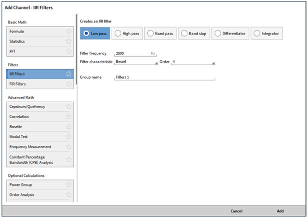
Fig. 266 Pop-up window for creating a (low or high pass) IIR filter channel
The following IIR-Filter parameters are available:
Filter Type: Low pass, High pass, Bandpass, Band-stop, Differentiator, Integrator
If Low pass or High pass filter is selected (see Fig. 266), the user can select
Filter Frequency: from 0 Hz to < Nyquist frequency (0.99 * sample rate) / 2
Filter Characteristic: Bessel, Butterworth, Chebyshev I or Chebyshev II (for Chebyshev filter, the Ripple (Stopband) can be defined from 0 to 80 dB)
Filter Order: 2, 4, 6, 8, 10
Group name: Define a group in the Channel List to which the filter shall be added.
If Bandpass or Bandstop filter is selected (see Fig. 266), the user can select
Low Frequency: from 0 Hz to < Upper frequency Hz
High Frequency: from (Lower frequency + 1) Hz to < Nyquist frequency. (0.99 * sample rate) / 2
Filter Characteristic: Bessel, Butterworth, Chebyshev I and Chebyshev II (for Chebyshev filter, the Ripple (Stopband) can be defined from 0 to 80 dB)
Filter Order: 2, 4, 6, 8, 10
Group name: Define a group in the Channel List to which the filter shall be added
If Differentiator is selected, the user can select
Operation: Single or double differentiation
If high frequencies shall be filtered
Filter Frequency: from 0 Hz < Nyquist frequency. (0.99 * sample rate) / 2
Filter Characteristic: Bessel, Butterworth, Chebyshev I and Chebyshev II (for Chebyshev filter, the Ripple (Stopband) can be defined from 0 to 80 dB)
Filter Order: 2, 4, 6, 8, 10
Group name: Define a group in the Channel List to which the filter shall be added
If Integrator is selected, the user can select
Operation: Single or double integration
If low frequencies shall be filtered
Filter Frequency: from 0 Hz < Nyquist frequency. (0.99 * sample rate) / 2
Filter Characteristic: Bessel, Butterworth, Chebyshev I and Chebyshev II (for Chebyshev filter, the Ripple (Stopband) can be defined from 0 to 80 dB)
Filter Order: 2, 4, 6, 8, 10
Group name: Define a group in the Channel List to which the filter shall be added
Note
Filters can only be applied to synchronous channels, such as analog input channels or counter channels but not to asynchronous channels, such as CAN channels, EPAD channels, or power group channels.
After pressing enter, the channel will appear in the Data Channels menu. The defined channel parameters can be changed afterwards in the Channel Setup (see Fig. 267).
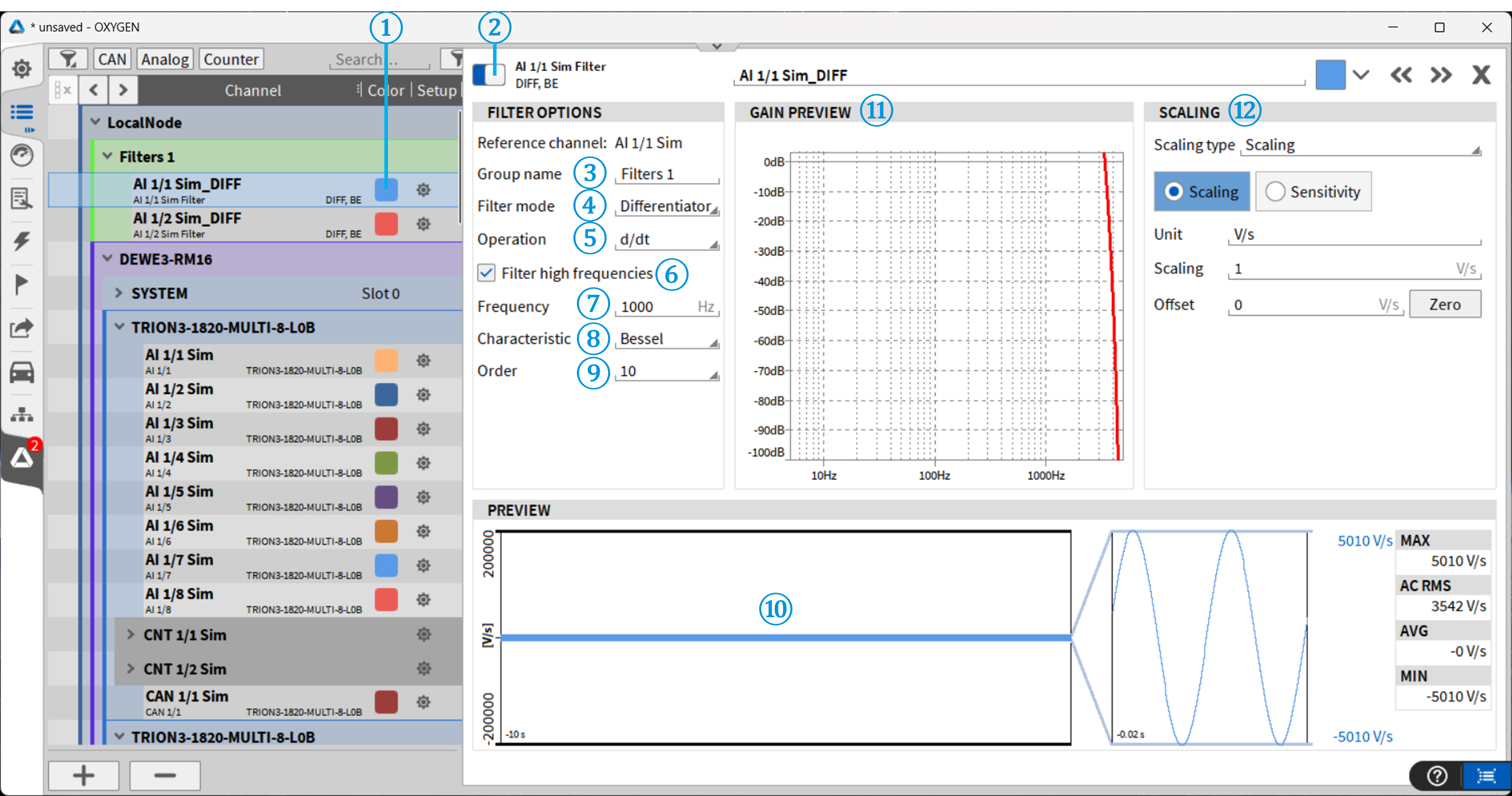
Fig. 267 Filter channel setup - overview
No. |
Function |
Description |
|---|---|---|
1 |
Color |
Color scheme of the channel can be changed here. |
2 |
Active button |
Setting a channel active or inactive; an active channel can be displayed in an instrument, used in a math channel and can be recorded, an inactive channel not. |
3 |
Group Name |
Name of IIR Filter group |
4 |
Filter Mode |
Select the filter type: Lowpass, High pass, Differentiator, Integrator |
5 |
Operation Setup |
Select the Operation type Single or Double Integration / Differentiation (only applicable for Differentiators and Integrators) |
6 |
Filter high frequencies |
|
7 |
Frequency |
Specify the cut-off frequency from > 0 to Nyquist frequency. (0.99 * sample rate) / 2 |
8 |
Characteristic |
Select between Bessel, Butterworth, Chebyshev I and Chebyshev II filter. |
9 |
Order |
Select a 2nd, 4th, 6th, 8th or 10th filter order. In case a Chebyshev is chosen a parameter for the ripple (passband) in DB is chosen. |
10 |
Preview window |
Real Time preview of the calculation |
11 |
Gain window |
Gain preview in dB up to < Nyquist based on sample rate. |
12 |
Scaling menu |
Change the channels’ scaling by entering a Scaling factor or changing the sensitivity (and/or entering an offset) or by a 2-point scaling |
FIR Filter channel
To create FIR filtered channels, click on the [+] button in the lower-left corner of the Data Channels menu (see Working with Software Channels) and select FIR Filters. Multiple channels can be selected at the same time to create multiple filter channels with the same settings.
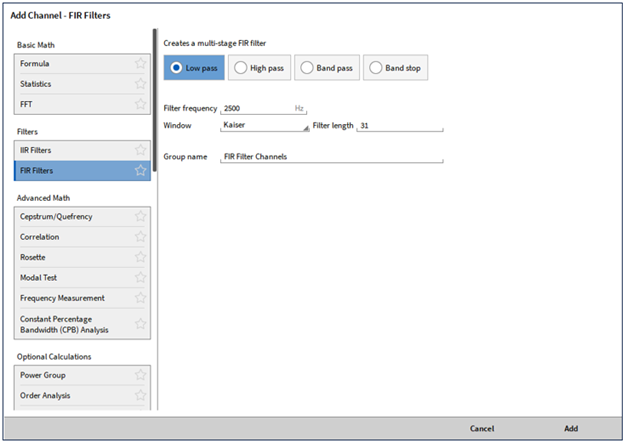
Fig. 268 Pop-up window for creating an FIR (low pass and bandpass) filter channel
After FIR Filter is pressed, the following filter characteristics can be selected:
Filter type: low pass, high pass, band pass, band stop.
If low-pass or high-pass filter is selected, the following can also be set:
Filter frequency: from 0 Hz to
 Hz, Default
Window mode: Kaiser, Rectangular, Hann, Hamming, Blackman, Blackmann/Harris, Flat Top, Bartlett, Cosine
Filter length: between 8 and 32768
Group name: define a group name in the channel list to which the filter should be added
When Bandpass or Bandstop is selected:
Lower frequency: from 0 Hz to < Upper frequency Hz
Upper frequency: from
 Hz
HzWindow mode: Kaiser, Rectangular, Hann, Hamming, Blackman, Blackmann/Harris, Flat Top, Bartlett, Cosine
Filter length: between 8 and 32768 (default = 31)
Group name: define a group name in the channel list to which the filter should be added
Note
Filters can be applied only to synchronous channels, like analog input channels or counter channels, but not to asynchronous channels, like CAN channels, EPAD channels or power group channels.
Pressing Add creates the filter channels in the channel list. All defined channel parameters can be modified later in the Channel Settings. In general, the FIR channel settings are divided into four sections:
FIR Filter Options – define and adjust the FIR configuration
FIR Stages – specify filter behavior; additional stages can be added using [+]
Input Channels – select the channels to be filtered
Preview – display the filter behavior
For a detailed description see Fig. 269 and Table 29.
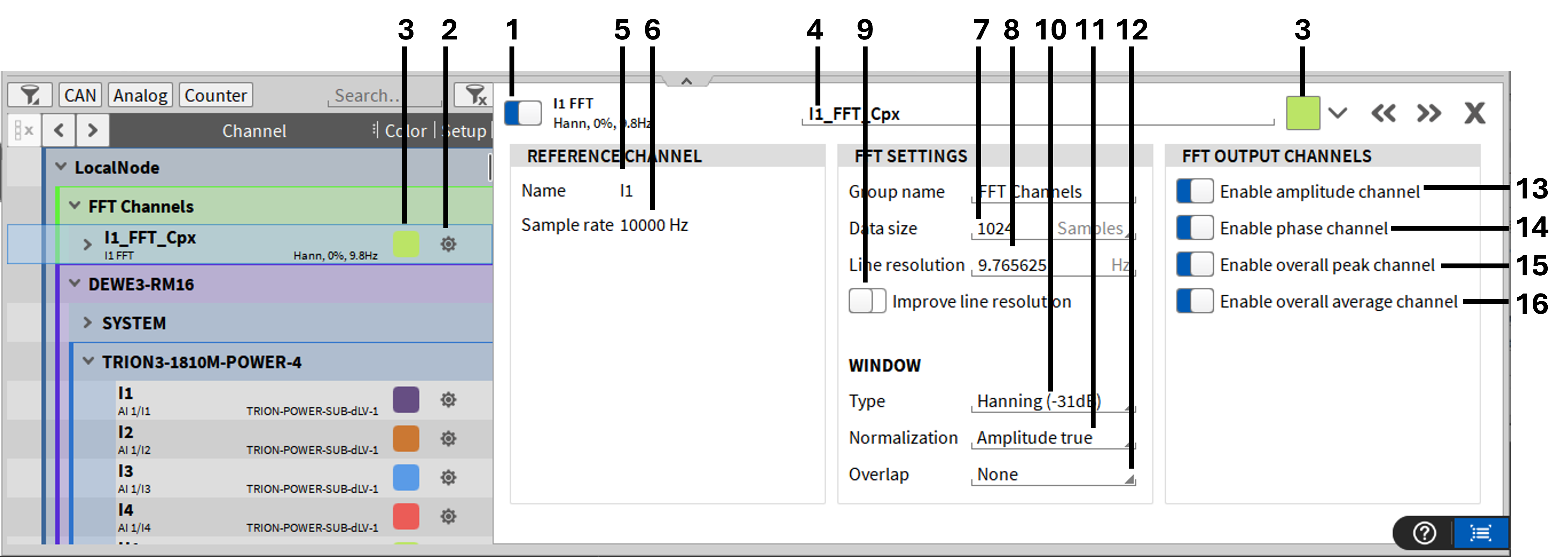
Fig. 269 FIR settings
Nr. |
Feature |
Description |
|---|---|---|
1 |
Color |
Color scheme for a channel can be changed here. |
2 |
Activate |
Enables or disables a channel. Deactivated channels are not displayed, not recorded, and cannot be used for further analysis. |
3 |
Group name |
Define the name of the channel group within the OXYGEN channel list |
4 |
Filter type |
Select the filter type: Lowpass, Highpass, Bandpass, Bandstop |
5 |
Filter length |
Between 8 and 32768 |
6 |
Window |
Kaiser, Rectangular, Hann, Hamming, Blackman, Blackman/Harris, Flat Top, Bartlett, Cosine |
7 |
Filter delay |
Delay depending on filter length and filter stages |
8 |
Compensate delay |
Automatically compensate filter delay Yes = TRUE, No = FALSE |
9 |
Saturation detection |
Enables (True) or disables (False) saturation detection. When enabled, and the input channel is saturated or exceeds the measuring range, the corresponding FIR channel outputs “NaN” for as long as saturation occurs (see Fig. 270). A channel is considered saturated once 99 % or 99.9 % (selectable)of the range (of the input channel) is reached. When disabled, the channel outputs the range limit value instead. |
10 |
Channel list |
List of available input channels. Select or deselect channels to be filtered. |
11 |
Channel filter |
Filters the channel list using multiple filter options. |
12 |
Channel grouping |
Displays the channel list sorted either by channel groups or alphabetically. |
13 |
Cutoff frequency |
Define the cutoff frequency; must satisfy 0 < fcutoff < input sample rate / 2 |
14 |
Decimation factor |
Reduces the output sample rate by the given factor – e.g. input sample rate: 10 kHz, decimation factor: 5 –> output sample rate: 2 kHz. In between samples are skipped. Available for low-pass filters only. |
15 |
Output sample rate |
Displays the resulting output sample rate. |
16 |
Preview |
Preview of filter behavior |
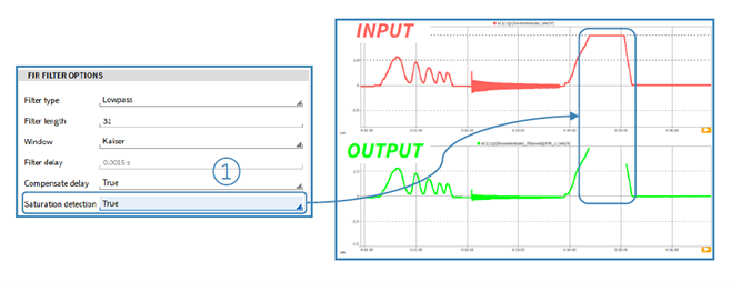
Fig. 270 FIR – Saturation detection
Choice of filter length:
A shorter filter length has fast execution times and therefore shorter delay times; however, choosing very short filter lengths results in a flat attenuation drop. The attenuation drop is displayed in the preview window when the filter lengths are changed.
The filter length can be defined with the following formula.
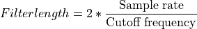
High attenuations in the stopband or low ripples in the passband may require a higher filter length. In the case of a low pass filter it makes sense to define several filter stages if the calculated filter length is too high. This happens, for example, if for a signal with a sampling frequency of 200 kHz, you are only interested in frequencies below 100 Hz. As a result, the individual filter stages are performed with lower filter lengths, which results in a reduction of the computational load.
Frequency tracking
In the filter options, you can create a bandpass filter with variable center frequency.
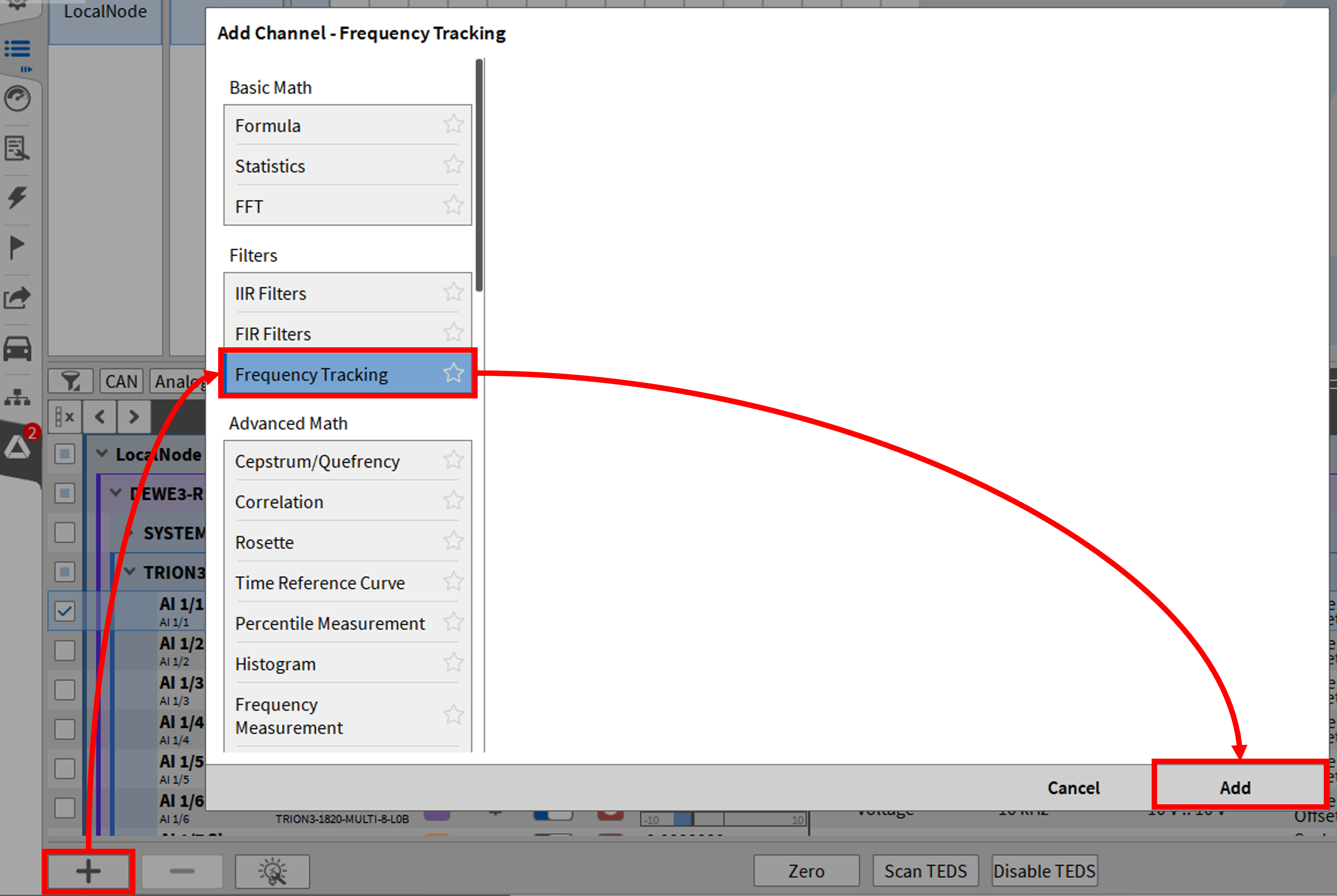
Fig. 271 Creating a frequency tracking filter
If channels were selected before creating the filter, the first selected channel is assigned as the reference channel, and all subsequent channels are assigned as input channels.
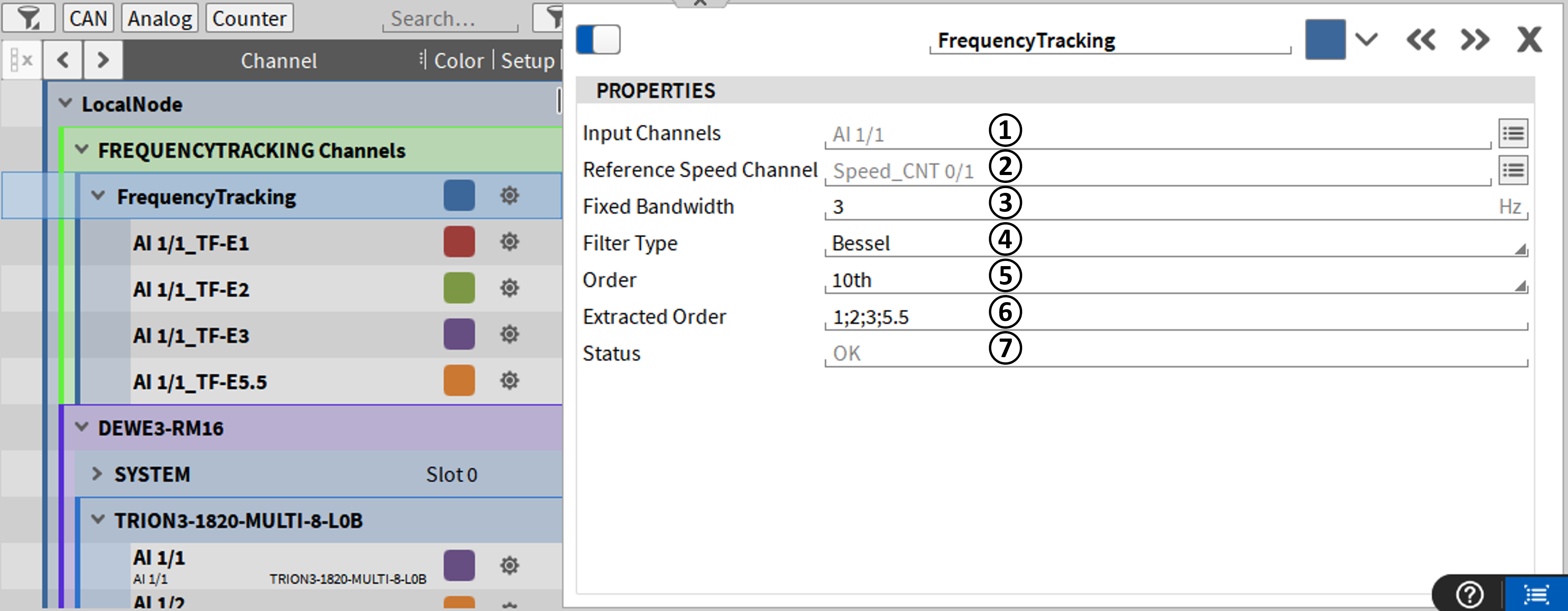
Fig. 272 Channel settings of the frequency tracking
Nr. |
Function |
Description |
|---|---|---|
1 |
Input channels |
One output channel per extracted order is created for the assigned input channels |
2 |
Reference speed channel |
The reference channel determines the center frequency of the bandpass filter. This can be specified in rpm or Hz. If there is a unit error, this is displayed in the status line ⑦. |
3 |
Fixed bandwidth |
The fixed bandwidth determines the frequency above and below the reference frequency at which the input signals are attenuated by 3 dB. Meaning for a fixed bandwidth of 3 Hz, the damping of frequencies which are 3 Hz above the reference frequency is -3 dB. |
4 |
Filter type |
Select the filter function, either Bessel or Butterworth. |
5 |
Order |
Determines the power of the filter function from 2nd to 10th order. |
6 |
Extracted order |
Determines the ratio to the reference frequency for which the bandpass filter is to be applied. Non-integer values are also possible. |
7 |
Status |
Potential errors in the channel units or sampling rates are displayed here. |
Advanced math
Cepstrum/Quefrency
Cepstrum is a signal processing algorithm introduced in the 1960s for audio and acoustic analysis. Originally, Cepstrum was used to separate excitation parameters from sound-affecting parameters.
Examples:
Speech: Excitation of the vocal cord and impairment of the oral cavity.
Stringed instruments: string excitation and body resonance
Cepstral analysis is nowadays also used for vibration analysis and can be used, for example, to characterize seismic echoes, such as those from earthquakes and bomb blasts. It is a non-linear Fourier method which is used to “deconvolve” two signals.
In general, Cepstrum analysis is performed in the following way (see Fig. 273):
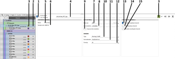
Fig. 273 Cepstrum analysis
The term “Cepstrum” is an artificial word, which is created from the word “Spectrum” by swapping the first four letters. In the same way “Frequency” becomes “Quefrency” and “Filtering” becomes “Liftering”. (see Fig. 273):
The algorithm is defined as follows. When measuring an acoustic signal, the signal is transformed into the frequency domain by means of FFT, then the natural logarithm of the spectrum is formed and finally transformed back into the time domain by means of an inverse FFT. The result of this algorithm is the cepstrum.
Use in OXYGEN
Clicking on “+” in the channel list opens the window for selecting the various math functions. Under the basic math functions there is the option to add a cepstrum/quefrency analysis. (see Fig. 274) It is possible to choose among 3 different cepstral analyses. You can choose between “Amplitude”, “Power” and “Complex”. Furthermore it is possible to activate a filtering (liftering) and to define a group name in which the new channels will be added to the channel list. (for more information on the functions, see Fig. 273) By clicking on the “Add” button in the lower right corner of the window, the created channels are automatically created to the defined group name.
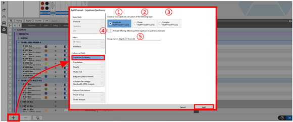
Fig. 274 Adding Cepstrum/Quefrency
Nr. |
Function |
Description |
|---|---|---|
1 |
Amplitude |
The amplitude cepstrum or real cepstrum is defined as follows:
|
2 |
Power |
In Power Cepstrum, the absolute value is squared before it is
logarithmized. The calculation is:
|
3 |
Complex |
With the complex spectrum, not the magnitude of the FFT, but the
complex spectrum is logarithmized. Thus, the phase info is
preserved during the reverse transformation. The calculation is:
|
4 |
Liftering |
When activated, the filtering is activated and can then be adjusted in the settings of the created channel. |
5 |
Groupname |
Defines the group name in which the generated channels of the cepstral analysis are listed. |


After clicking on “Add”, a new Cepstrum group is added under the specified group name. By opening the properties of the newly created group, further settings for the cepstral analysis can be made (see Fig. 275). In addition to the “Liftering channels”, 3 further channels are automatically created and are thus available to you.
Cepstrum: This is the continuous Cepstrum
Overall: The total Ceptrsum averaged from the start of measurement to the end of measurement.
Spectrum: The logarithmized signal in the frequency domain
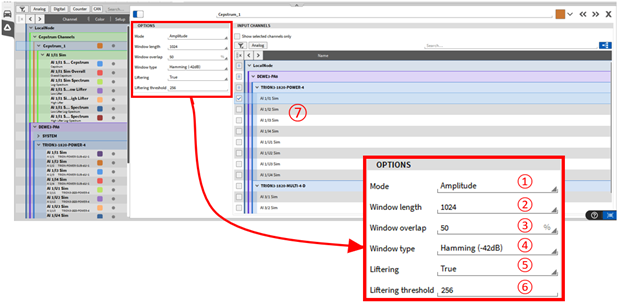
Fig. 275 Cepstrum settings
Nr. |
Function |
Description |
|---|---|---|
1 |
Mode |
The choices are: Amplitude, Power and Complex. |
2 |
Window length |
Select the number of samples to be simultaneously transformed into the frequency domain. The window width can vary between 32 and 262144 (218) samples. For more details on the calculation, see Instruments and instrument properties. |
3 |
Window overlap |
Select an overlap factor between 0 to 90 %. For more details, see Calculation of the Periodogram - Averaging of FFT windows. |
4 |
Window type |
Choose a suitable window. The choices are: Hanning, Hamming, Rectangle, Blackman, Blackman-Harris, Flat Top or Bartlett. For more details of the calculation, see Window type. |
5 |
Liftering |
Here the liftering (filtering) can be activated or deactivated. |
6 |
Liftering threshold |
Here you can enter a limit value in samples. The cepstrum is thus divided into an upper (H) and lower (L) cepstrum. All cepstrum samples below the limit value (incl. limit value) are written into a new channel “Low-Lifter”. - Output channel Low-Lifter-Spectrum: Re{ FFT(L * Cepstrum) } - Output channel Low-Lifter: Re{ IFFT(exp(FFT(L * Cepstrum))) } All cepstrum samples above the threshold (excl threshold) are written to a new channel “High-Lifter”. - Output channel High-Lifter-Spectrum: Re{ FFT(H * Cepstrum) } - Output channel High-Lifter: Re{ IFFT(exp(FFT(H * Cepstrum))) } This applies to amplitudes and power cepstrum. For the complex cepstrum, the absolute value of the complex signal is always output instead of the real part. |
7 |
Channel selection |
Here you can select the channels for which a cepstral analysis has to be performed. |
Correlation
Clicking on “+” in the channel list opens the window for selecting the different math functions. Under the basic math functions there is the option to add a correlation (see Fig. 276 ). It is possible to choose between an Auto or a Cross-correlation. Then press the “Add” button in the bottom right corner of the window and a new correlation channel will automatically be added to the channel list under the specified group name (see ③ in Fig. 276).
Auto-correlation
The Auto-correlation (see ① in Fig. 276) mathematically describes the convolution of a signal with itself and is used to detect periodicity in signals, e.g. in modulated and noisy signals.
Formula Auto-correlation:

The calculation is performed as follows:
Take a time signal and proceed block by block as follows:
FFT calculation
Multiplication of the spectrum with itself
Inverse FFT
Normalization to amplitude +/-1
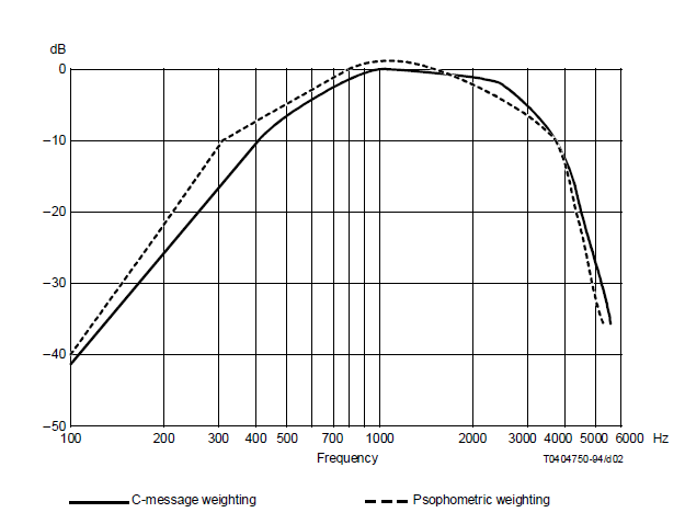
Fig. 276 Adding Auto and Cross-correlation
Settings of the Auto-correlation
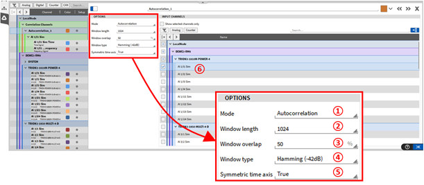
Fig. 277 Auto-correlation – settings
Nr. |
Function |
Description |
|---|---|---|
1 |
Mode |
The choices are: Auto-correlation and Cross-correlation. Here you can also switch between both calculations afterwards. |
2 |
Window length |
Select the number of samples to be simultaneously transformed into the frequency domain. The window width can vary between 32 and 262144 (218) samples. For more details of the calculation, see Instruments and instrument properties. |
3 |
Window overlap |
Select an overlap factor between 0 to 90 %. For more details, see Calculation of the Periodogram - Averaging of FFT windows. |
4 |
Window type |
Choose a suitable window. The choices are: Hanning, Hamming, Rectangle, Blackman, Blackman-Harris, Flat Top or Bartlett. For more details of the calculation, see Window type. |
5 |
Symmetric time axis |
Visualization of the autocorrelation either from -t/2 … +t/2 (True) or 0 … t (False). |
6 |
Channel selection |
Here you can select the channels for which an Auto-correlation is to be performed. |
Generated channels of the Auto-correlation
When you perform an autocorrelation, OXYGEN will automatically create 2 channels for you:
Time - The result of the autocorrelation in the time domain.

Frequency - The result of multiplying signal x by itself in the frequency domain
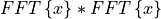
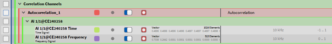
Fig. 278 Auto-correlation generated channels
Cross-correlation
The Cross-correlation (see ② in Fig. 276) mathematically describes the convolution of a signal x with another signal y. The Cross-correlation is used e.g. to detect identical components in 2 different signals or to analyze the delay time between 2 signals.
Formula Cross-correlation:

The calculation is performed as follows:
Take a time signal and proceed block by block as follows:
FFT calculation
Multiplication of the spectrum of signal x with the spectrum of signal y
Inverse FFT
Normalization to amplitude +/-1
Settings of the Cross-correlation
Fig. 279 Cross-correlation - settings
Nr. |
Function |
Description |
|---|---|---|
1 |
Mode |
The choices are: Auto-correlation and Cross-correlation. Here you can also switch between both calculations afterwards. |
2 |
Reference channel |
Select a reference channel for the calculation of the Cross-correlation. To do this, drag and drop the desired reference channel from the channel list ⑦ into the field for the reference channel ②. |
3 |
Window length |
Select the number of samples to be simultaneously transformed into the frequency domain. The window width can vary between 32 and 262144 (218) samples. For more details, see Instruments and instrument properties. |
4 |
Window overlap |
Select an overlap factor between 0 to 90%. For more details, see Calculation of the Periodogram - Averaging of FFT windows. |
5 |
Window type |
Choose a suitable window. The choices are: Hanning, Hamming, Rectangle, Blackman, Blackman-Harris, Flat Top or Bartlett. For more details of the calculation, see Window type. |
6 |
Symmetric time axis |
Visualization of the autocorrelation either from -t/2 … +t/2 (True) or 0 … t (False). |
7 |
Channel selection |
Here you can select the channels for which a Cross-correlation is to be performed, referring to the selected reference channel ②. |
Generated channels of the Cross-correlation
When you perform a cross-correlation, OXYGEN will automatically create 3 channels for you:
Time - The result of the cross-correlation in the time domain.

Frequency - The result of the multiplication of signal x and signal y in the frequency domain
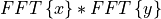
Coherence
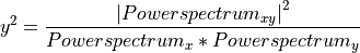
The coherence is an indicator to see if the reference signal x and the signal y match. The more identical the two signals are, the closer the value is to 1. If the signals are exactly identical, the coherence would return “1” as a result.
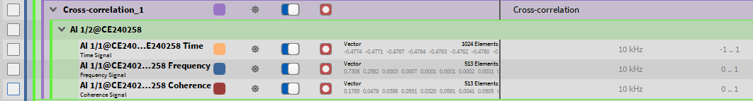
Fig. 280 Cross-correlation generated channels
Rosette (strain gauge) channels
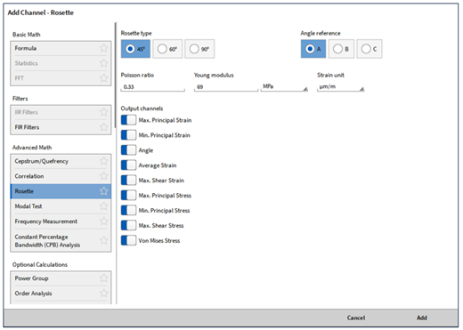
Fig. 281 Pop-up window for creating a Rosette calculation
For creating a Rosette channel, the user must click on the Add button in the lower left corner (marked red in Fig. 224) and a window will appear (see Fig. 281). To create a Rosette channel, select Rosette. After clicking on the OK button, a Rosette main channel (Rosette_1 in Fig. 282) with its Sub channels (Max Principal strain to VonMises Stress in Fig. 282) is added to the channel List. A click on the gear button of the main rosette channel will open the Rosette settings to perform changes afterwards (see Fig. 282).
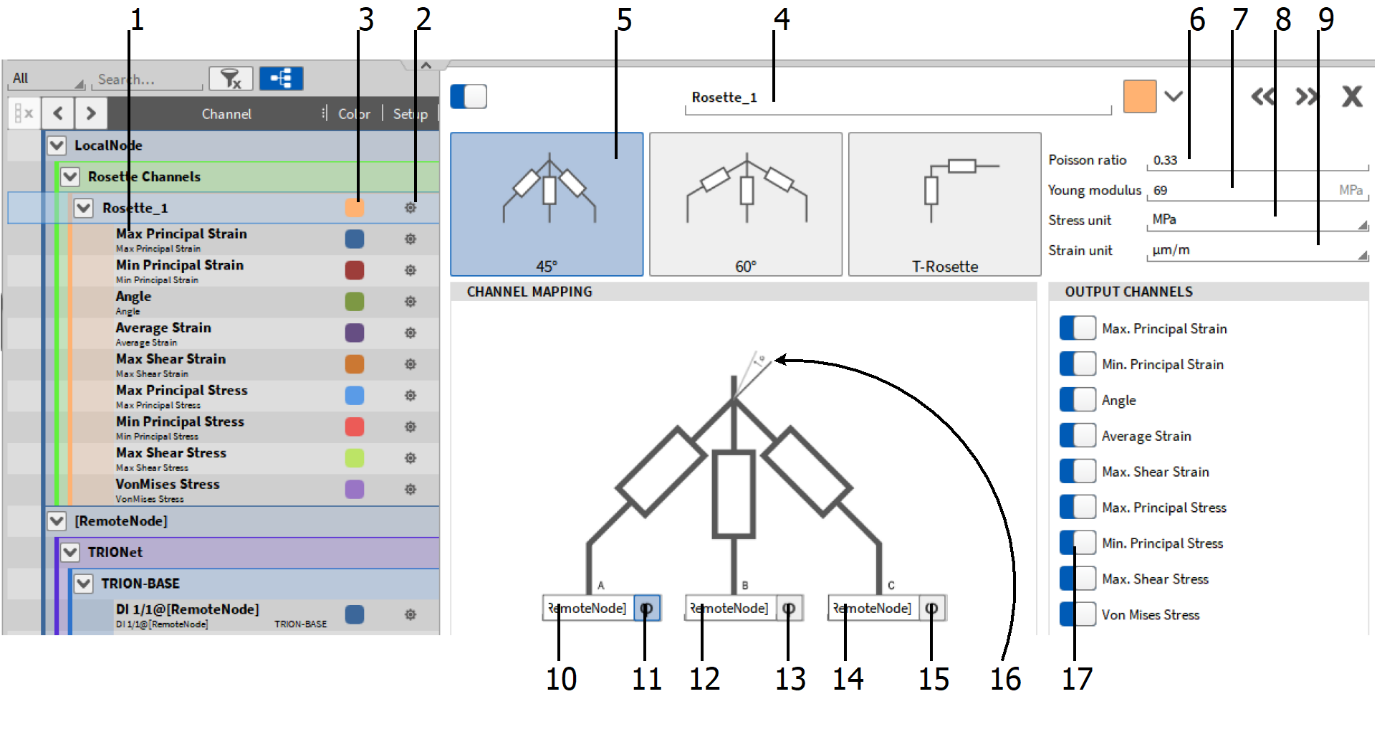
Fig. 282 Rosette channel setup – overview
No. |
Function |
Description |
|---|---|---|
1 |
Channel List |
Channel List including the output channels of the Rosette calculation. |
2 |
Channel setup button |
Opens the channel setup of the individual channel. |
3 |
Color |
Color scheme of the channel can be changed here. |
4 |
Channel Name |
Individual channel name; Can be changed individually. |
5 |
Rosette Type selection |
Select the rosette calculation type here: 45°, 60°, 90° (T). |
6 |
Poisson ratio selection |
Enter the poisson ration here. |
7 |
Young modulus selection |
Enter the Young modulus of the used material here. |
8 |
Stress unit selection |
Select the unit of the Young modulus here: [MPa], [GPa] or [kgf/mm2]. |
9 |
Strain unit selection |
Select the strain unit here: [µm/m] or [microstrain]. |
10 |
Epsilon A channel assignment |
Assign the input channel for Epsilon A here. |
11 |
Reference Angle Selection |
Select Epsilon A as Reference Angle here; If selected, the background will highlight grey-blue. |
12 |
Epsilon B channel assignment |
Assign the input channel for Epsilon B here. |
13 |
Reference Angle Selection |
Select Epsilon B as Reference Angle here; If selected, the background will highlight grey-blue. |
14 |
Epsilon C channel assignment |
Assign the input channel for Epsilon C here. |
15 |
Reference Angle Selection |
Select Epsilon C as Reference Angle here; If selected, the background will highlight grey-blue. |
16 |
Reference Angle hint |
Highlights the selected reference angle in the rosette schematics. |
17 |
Output channel activation |
Activate or deactivate the single channels that shall be calculated and output by the calculation. |
Required input channels
The Plugin requires three strain gauge input channels (Epsilon A, B, C), the angular rosette alignment (45°, 60°, 90° (T)) and the angle reference (A, B, C). Available input channels for Epsilon A, B, C are analog input channels. The 90° or Tee type rosette requires only 2 input channels (Epsilon A, B).
The advantage of using three-channel rosettes is to minimize the effect of error due to misalignment to the elements from the physical axis. Furthermore, the bigger the angle between the gauges, the better the result concerning noise influence.
Note
Channels that are assigned to the Rosette plugin require the engineering unit µm/m or um/m. Other engineering units are not accepted and will lead to the error message Unit of input channels not µm/m or um/m in the Channel Setup of the main rosette channel (see Fig. 283).
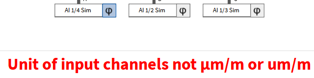
Fig. 283 Error message in case of wrong engineering unit
The channel to be used for the rosette calculation can be selected before clicking on the Calculator button. If channels 1/1, 1/2 and 1/3 are selected one after the other and a three channel is selected, the channels will be assigned automatically in the following manner after clicking the OK button in the Rosette Calculation Setup: 1/1 to Epsilon A, 1/2 to Epsilon B and 1/3 to Epsilon C.
If channels 1/3, 1/1 and 1/2 are selected one after the other and a three channel is selected, the channels will be assigned automatically in the following manner after clicking the OK button in the Rosette Calculation Setup: 1/3 to Epsilon A, 1/1 to Epsilon B and 1/2 to Epsilon C
If six channels 1/1, 1/2, 1/3, 1/4, 1/5 and 1/6 are selected one after the other, two three-channel rosettes or three two-channel rosettes can be created with one click on the Calculator button. The input channels will be assigned in the following manner (example for two three-channel rosettes):
Rosette 1: 1/1 to Epsilon A, 1/2 to Epsilon B and 1/3 to Epsilon C
Rosette 2: 1/4 to Epsilon A, 1/5 to Epsilon B and 1/6 to Epsilon C
If four channels1/1, 1/2, 1/3, 1/4 are selected one after the other and two three-channel rosettes shall be created, the input channels will be assigned in the following manner:
Rosette 1: 1/1 to Epsilon A, 1/2 to Epsilon B and 1/3 to Epsilon C
Rosette 2: 1/4 to Epsilon A, Epsilon B and Epsilon C will remain unassigned
The channel assignment can be edited after creating the Rosette calculation in the Channel setup of the main channel (see ⑯ in Fig. 282) by dragging and dropping the desired channel from the Channel List on the left-hand side to the individual input channel of the rosette calculation (see Fig. 284).
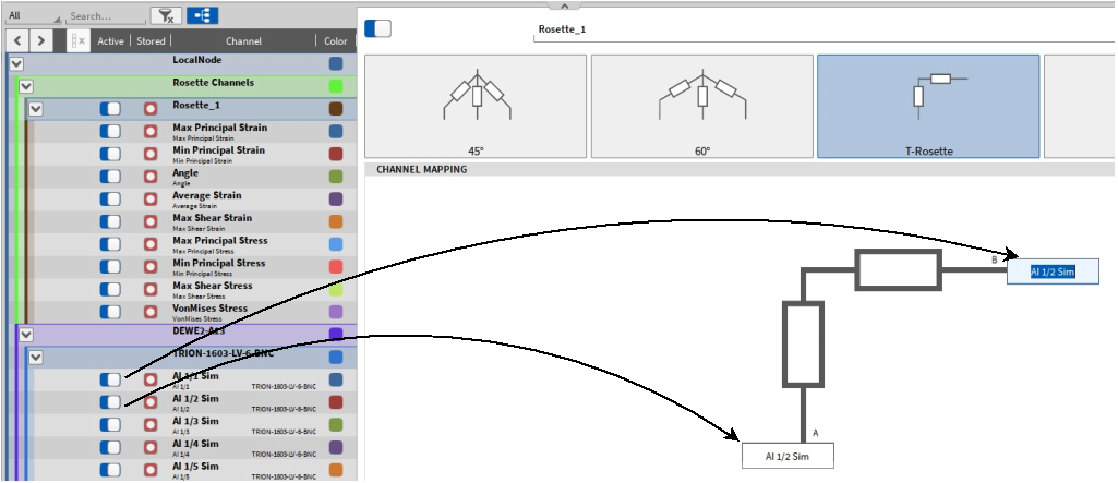
Fig. 284 Channel assignment in the rosette channel setup
If the assignment of a rosette input channel is missing, the error message Input channels not ready will be displayed at the bottom of the Channel Setup (see Fig. 285).

Fig. 285 Error message in case of missing channel assignment
The sample rate of the channels assigned to one rosette calculation must all be same . If they differ, the error message Sample rates of input channels differ will be displayed at the bottom of the Channel Setup (see Fig. 286).

Fig. 286 Error message in case of different channel sample rates
The sub channels (see ⑰ in Fig. 282) resulting from the rosette calculation have a Channel Setup that can be accessed via the Gear Button in the Channel List as well. But only the Channel scaling can be edited there.
Resulting output channels
The plugin uses the so-called Mohr’s circle (see Mohr’s circle) for the calculations. For details, refer to the relevant literature.
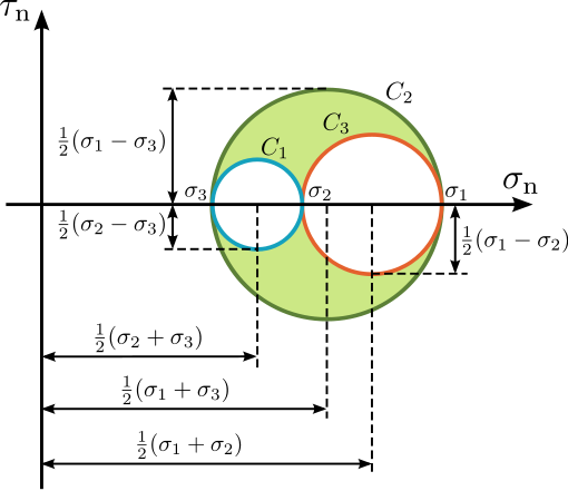
Fig. 287 Mohr’s circle
The calculated values are represented in channels, which are shown below.
Max Principle Strain → Max. Strain in angle direction [µm/m] or [microstrain]
Min Principle Strain → Min. Strain in angle +90° direction [µm/m] or [microstrain]
Angle → Angle of max. strain [°]
Average Strain → Center of Mohr’s circle [µm/m] or [microstrain]
Max Shear Strain → Radius of Mohr’s circle [µm/m] or [microstrain]
Max Principle Stress → Max. stress in angle direction [MPa]
Min Principle Stress → Min. stress in angle +90° direction [MPa]
Max Shear Stress → Max. shear stress in angle direction [MPa]
Von Mises Stress → Virtual uniaxial stress [MPa]
Usage of the plugin
The Rosette Math plugin is used to determine the angle and max/min amplitude of strain and stress on a surface. This is used when it is not known which direction of strain/stress has to be expected.
Rosette strain gauges are available combined in one foil (stacked construction), alternatively it is possible to use three separate strain gauges (planar construction).
Fig. 288 shows sketches of different rosette types: left: 90° (T), middle: 45°, right: 120° rosette.
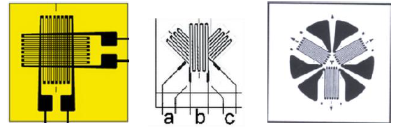
Fig. 288 Sketch of different rosette types
Physical basics
This chapter includes some important term explanations.
Strain : Is the mechanical deformation measured as a relation between length change relative to the initial length:
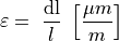
The strain is usually presented in µm/m, so the ratio of elongation is micrometers comparing to the length of a specimen in meters. So, what does that mean if we measure a value of 2000? First of all, we can also express this in percent. Strain in
 /m divided by a factor of 10000 results in elongation in percent. In the case of 2000, the elongation will be 0.2 %.
Stress : Is defined as the average force per unit area, also taking in account the material.
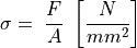
Young’s modulus: The formulas shown above only work in the linear part of the Strain-Stress-Curve, which is shown in Fig. 289. In this area a constant factor between stress and strain exists.
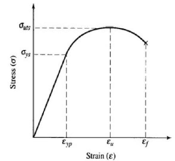
Fig. 289 Strain-Stress-Curve
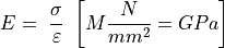
Where Е is the Young’s modulus or Elastic modulus. This constant is depending on the used material (e.g. steel = 210 kN/mm2). The measured value from the strain gauge is therefore the strain and you get the stress by calculating .
Implemented formulas
The Rosette calculations depend on the selected rosette type and angle reference.
Constants


Angle Reference


Calculation of 45° and 90° Rosette
Avg Strain
MaxShearStrain


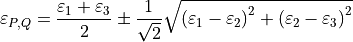
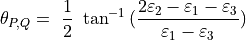
Calculation of 60° and 120° Rosette

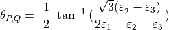
Calculations valid for all Rosette types
Max/Min Principle Stress
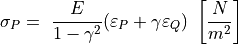
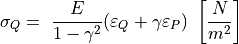
Von Mises Stress
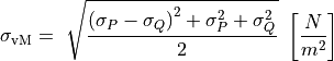
Max Shear Stress
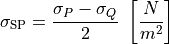
Addition to Angle Calculation
The following table shows how to determine the principal axis angle φ0 taking the sign of the numerator and the enumerator into account
Quadrant |
Z |
N |
Angle φ0 |
|---|---|---|---|
I |
+ |
+ |
0° ≤ φ0 ≤ +45° |
II |
+ |
- |
+45° ≤ φ0 ≤ +90° |
III |
- |
- |
-45° ≤ φ0 ≤ -90° |
IV |
- |
+ |
0° ≥ φ0 ≥ -45° |
Time reference curve
In OXYGEN, a time reference curve can be created in the Advanced Math options. This serves as a purely visual reference and can be used like other channels in the recorder, etc.
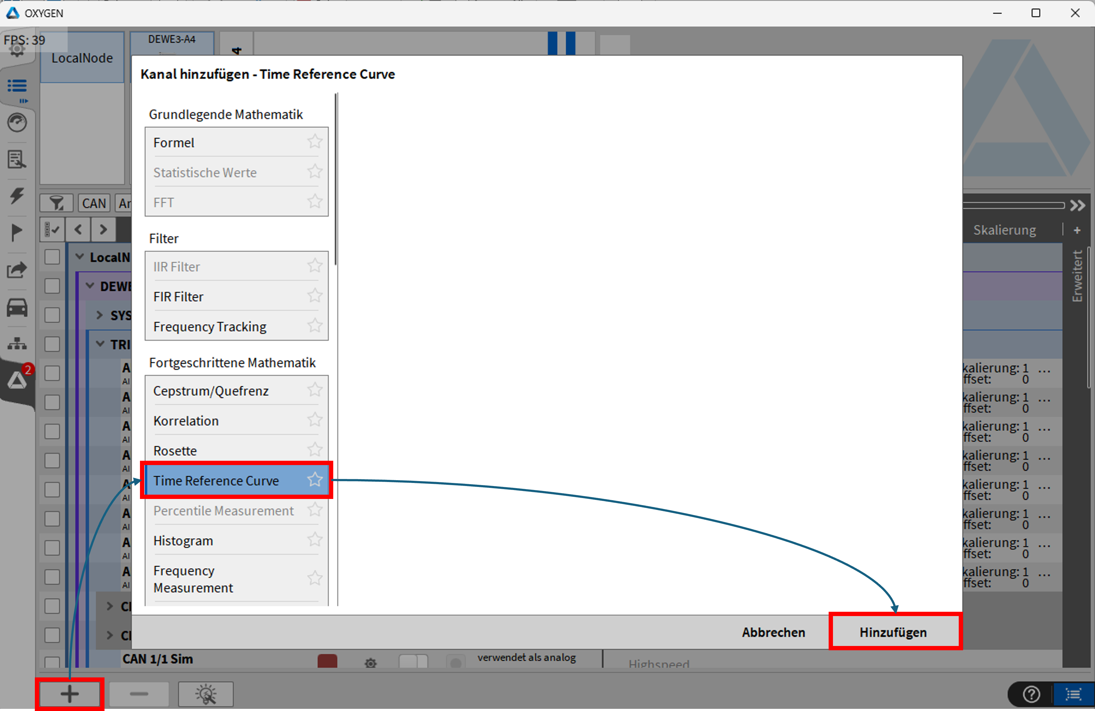
Fig. 290 Creating a time reference curve
After creating the reference curve, settings can be defined for, among other things, the type, i.e., whether one or two curves should be created, and the data source, i.e., whether a table or another measurement file should determine the curves. The other options are explained in more detail in Table 36. In the following figure, Fig. 291, two reference curves, Upper/Lower, was selected as type, the data source is a Table and the start on condition is On Channel.
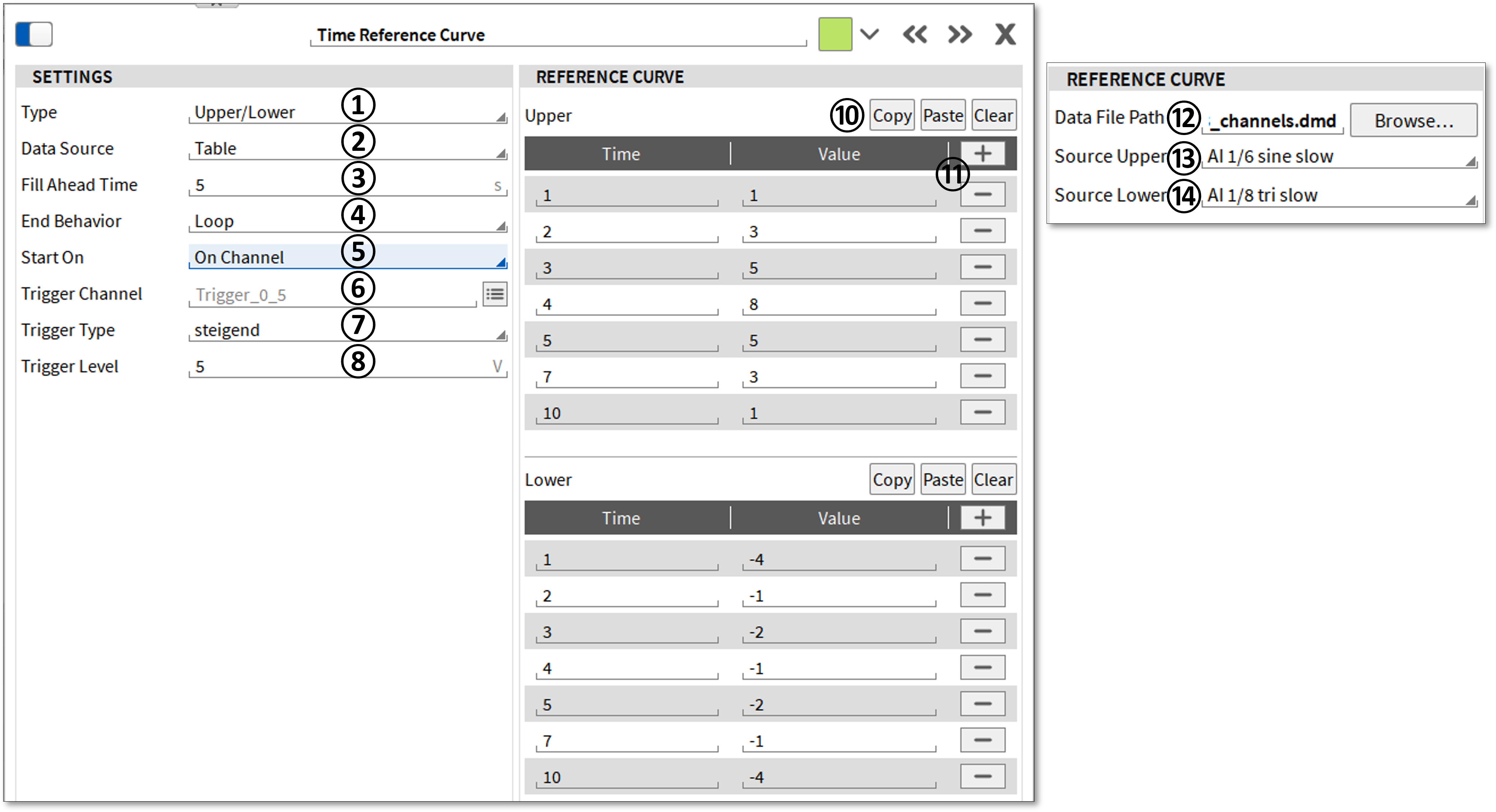
Fig. 291 Properties of the time reference curve
Nr. |
Name |
Description |
|---|---|---|
1 |
Type |
Select whether to create one (Single) or two (Upper/Lower) reference curves. |
2 |
Data Source |
Select what should be the basis for the reference curve. Either a Table with time and value or based on channel from Data file. |
3 |
Fill Ahead Time |
A time offset for the reference curve can be set here. This means that the reference curve begins 0…500 s before the current time, see Fig. 292. |
4 |
End Behavior |
Select whether the reference curve should be completely repeated after the data points have been processed: Loop, hold the last data point – Repeat Last Value or do not continue – NaN. |
5 |
Start On |
There are three options for starting the reference curve. Start On Channel means that the start of the curve is triggered by a channel. Start On Acquisition means that the reference curve starts when data acquisition begins (without measurement). Start On Measurement means that the reference curve starts when the measurement is armed. If the start condition is not met, the first value of thereference curve is repeated. |
6 |
Trigger Channel |
Only available for start condition On Channel selection. Select the trigger channel for starting the reference curve. This can be either math channels or analog channels. |
7 |
Trigger Type |
Only available for start condition On Channel selection. Select whether the reference curve should start when the trigger level ⑧ is exceeded or not reached. |
8 |
Trigger Level |
Only available for start condition On Channel selection. Selection of the level at which the start condition is met. |
9 |
Rearm Level |
Only available for start condition On Channel selection. Selection to define the level required to start the reference curve again on trigger. |
10 |
Reference curve Copy/Paste/Clear |
If a data file has been selected as the data source, the data points can be defined either in OXYGEN or in a third-party text editor. To export the table from OXYGEN, use Copy. To import the table from a text editor, use Paste. The structure is “Time in s” ‘Tab’ “Value.” The table can be deleted with Clear. |
11 |
Reference curve Plus/Minus |
Here, lines can be added (+) or deleted (-) for the reference curve. |
12 |
Datafile path |
If Table has been selected as the data source, an OXYGEN measurement file *.dmd can be selected to define the reference curves. |
13 |
Source Upper |
Select the channel for the upper reference curve from the measurement file selected in ⑫. |
14 |
Source Lower |
Select the channel for the lower reference curve from the measurement file selected in ⑫. |
The next figure Fig. 292 shows an example for an Upper- and Lower-time reference curve with a 5s pre time and the loop end behavior.
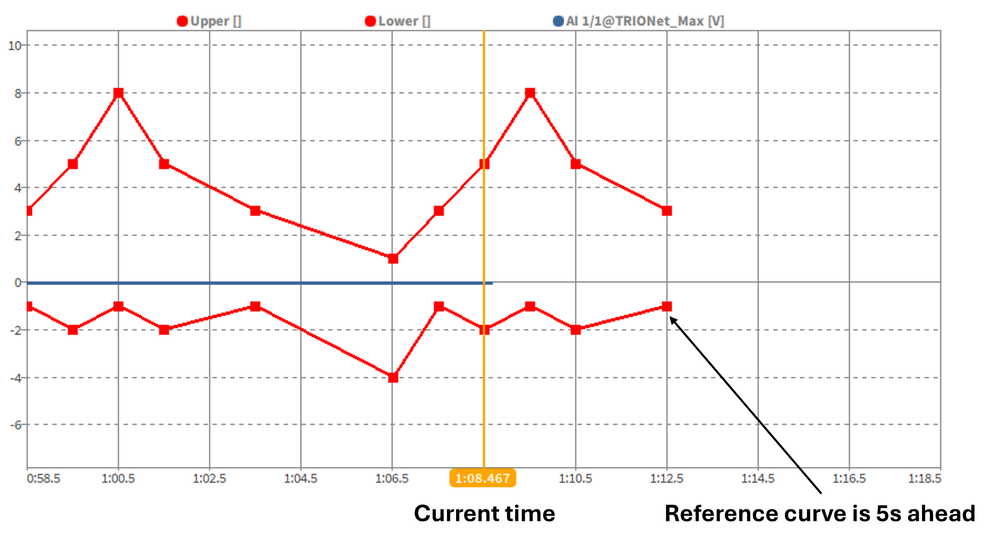
Fig. 292 Example for Upper and Lower Time Reference Curve with 5 s pre time (Fill ahead time)
Percentile
This module can be used to add a percentile measurement based on a synchronous or asynchronous time-dependent channel or array. With this calculation it is possible to calculate the threshold value that is exceeded in x% of the measurement time.
To create one or more channels for a percentile measurement, click on the + button in the bottom left corner of the channel list. A pop-up window appears in which the percentile measurement must be selected in the list (see Fig. 293). One or more channels must be selected in the channel list before clicking on the + button (see ① in Fig. 293). It is also possible to add channels for the measurement afterwards (see ① Fig. 294). You can specify 1 or more threshold values in %. When selecting multiple threshold values, the individual values must be separated by “;” (see ② in Fig. 293).
After clicking the Add button, a new section appears in the channel list called PERCENTILE MEASUREMENT Channels. To change the settings afterwards or to add channels or thresholds, click on the small cogwheel (see Fig. 294).
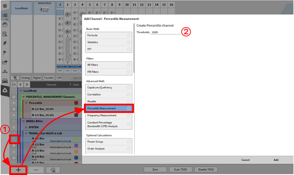
Fig. 293 Add a percentile measurement
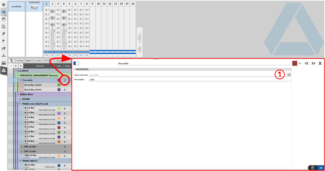
Fig. 294 Subsequent changes to the percentile measurement
During the measurement, the values for the percentile measurement are continuously recalculated, but only the last calculated value is saved in the measurement file (*.dmd) and is then available as a single value.
Histogram
The histogram is a math function for the statistical evaluation of a single channel. It can be found in the Advanced Math options (see Fig. 295).
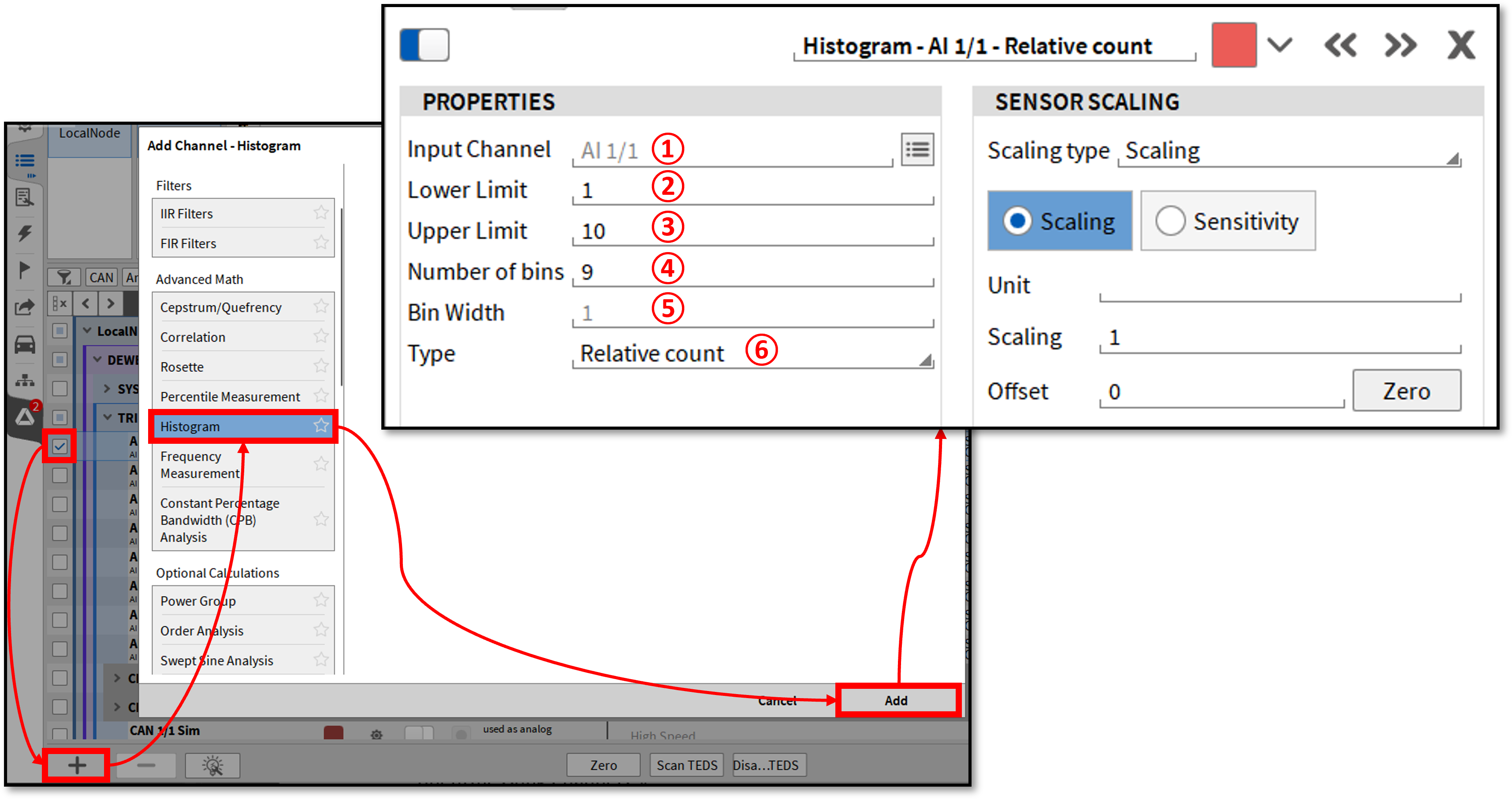
Fig. 295 Creation and configuration of a Histogram
No. |
Function |
Description |
|---|---|---|
1 |
Input channel |
Selection of channel for which a histogram calculation is to be performed. |
2 |
Lower limit |
Minimum value for creating the histogram; values below the limit are ignored. |
3 |
Upper limit |
Maximum value for creating the histogram; values above the limit are ignored. |
4 |
Number of bins |
The number of bins (intervals) displayed on the X-axis. |
5 |
Bin width |
The resulting width of the bins is from the limits and number of bins. (upper limit - lower limit) / number of bins |
6 |
Histogram type |
The histogram type defines the output (amplitude) of the calculation and the information stored in the output channels. The following types are available for selection: Absolute number, Relative number and Relative number in [%], Density and Density in [%], Distribution and Distribution in [%] |
Histogram type descriptions:
Absolute count: Each bin contains the number of measured values within the bin (the value is always counted upwards)
Relative count: Each bin value is the number of samples within the bin, normalized to the total number of samples counted (the sum of all bins is always 1)
Relative count [%]: Same as relative count, but expressed as a percentage (the sum of all bins is always 100)
Density: With empirical probability density, each relative count is divided by the bin width. In this case, the value is not dependent on the number of bins within a range
Density [%]: Same as density but expressed as a percentage (multiplied by 100).
Distribution: In an empirical probability distribution, the relative count is cumulated for each bin. This means that each bin is the sum of all lower bins and the current bin. The highest bin has the value 1.
Distribution [%]: Corresponds to the distribution but is expressed as a percentage. The highest bin has a value of 100.
An example is the following histogram with 13 bins, a lower limit of 1, and an upper limit of 10 is shown in Fig. 296. The signal has a maximum value of 8 V, meaning all bins above 8 show no relative count and density, but still a distribution of 1.
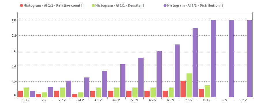
Fig. 296 Example of a Histogram with relative count, density and distribution
Frequency measurement
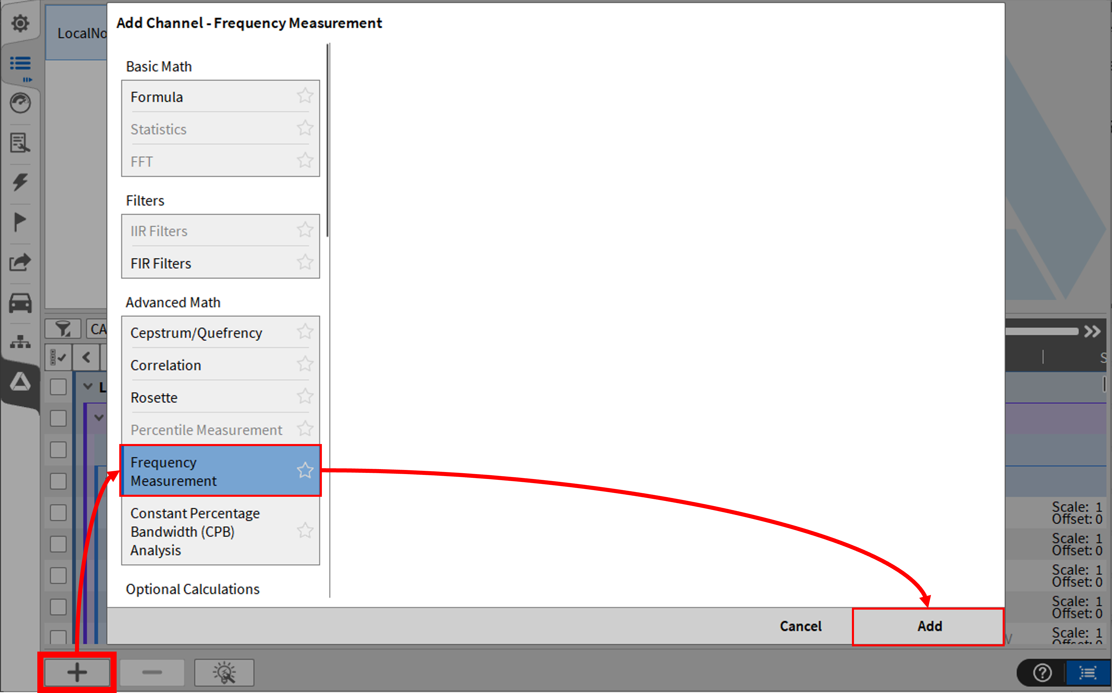
Fig. 297 Pop-up window for creating a frequency measurement channel
With this module it is possible to calculate the frequency of a periodical signal. The calculation is based on a block-wise calculation. To create one or several Frequency Measurement Channels click on the + button in the lower left corner of the channel list menu. A pop-up window will appear (see Fig. 297) where Frequency Measurement must be selected. The user can select several input channels simultaneously to create several frequency calculations before clicking on the + button or choose the channels after creating the Frequency Measurement channel.
After clicking on the Add button a new section in the channel list appears named Frequency Measurement Channels.
When clicking on the little gear button the settings of the frequency channel will open.
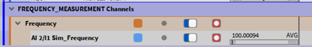
Fig. 298 Frequency Measurement Channels in Channel List
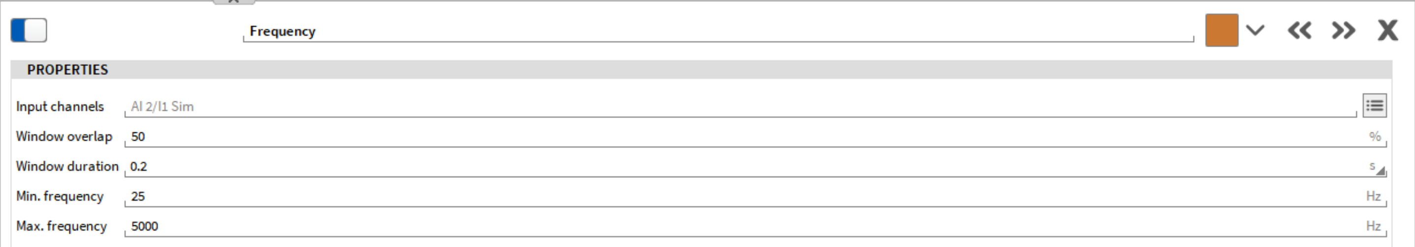
Fig. 299 Frequency Measurement Channel settings
The following settings are available:
Input channels: the input channels for the calculation can be selected when clicking on the button; a small pop-up window will appear where the desired channels can be changed or selected.
Window overlap: the window overlap can be entered here from 0 to 90 %.
Window duration: the window duration can be entered in this field, or a value can be chosen from the dropdown list; the minimum window duration is 10 ms up to 1 s.
Min. frequency: the minimum frequency which should be calculated must be entered here; the minimum frequency is 0 Hz.
Max. frequency: the maximum frequency is half the sample rate to account (Nyquist frequency).
CPB analysis
This is a standard feature and requires no additional license.
The CPB analysis computes a constant percentage bandwidth spectrum according to EN 61260 in Octave, Third octave or Twelfth octave resolution.
Creating a CPB Analysis
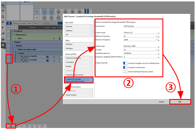
Fig. 300 Creating a CPB Analysis
Go to the Channel List and select one or several channels by checking their check boxes and press the + button
Select CPB Analysis, choose the proper calculation options and enable the required output channels (Details can be found in CPB analysis options)
Press Add afterwards to create the calculation. The channels will be added to the Channel List (see ④ in Fig. 301)
The settings can be accessed afterwards by clicking on the Gear button of the channel (see ⑤ in Fig. 301)
An Array Chart instrument can be used for visualizing the CPB spectrum. Further details can be found in Array Chart with Total column included.
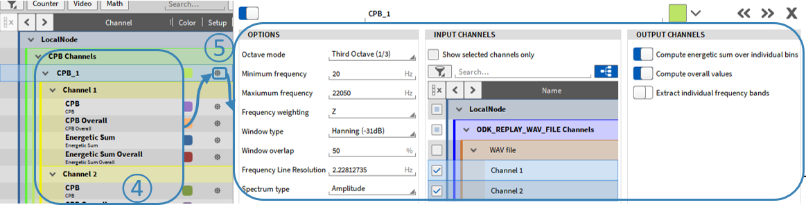
Fig. 301 CPB Analysis with extracted 100 Hz and 250 Hz bin
CPB analysis options
The following options can be selected for a CPB Analysis (see ② in Fig. 300):
Group Name: Set a group name for the actual calculation which appears in the Channel List
Octave mode: Select Octave, Third octave or Twelfth octave resolution (grouping according to EN 61260)
Minimum Frequency: Set a minimum frequency for computation. If the selected frequency is not the center frequency of a CPB bin, the bin including this frequency will be used as minimum bin.
Maximum Frequency: Set a maximum frequency for computation. If the selected frequency is not the center frequency of a CPB bin, the bin including this frequency will be used as maximum bin. The maximum frequency which can be set is 500 kHz.
Window type: Select between Hamming, Hanning, Rectangular, Blackman, Blackman-Harris, Flattop, Flattop-Bartlett Window for the spectral analysis
Overlap: Select an overlapping factor from 0 … 90 % for the spectral analysis
Amplitude Spectrum: Select between Amplitude spectrum or Decibel spectrum with freely definable reference value and corresponding reference level
Frequency Weighting: Select between frequency weighting according to DIN-EN 61672: A-, B-, C-, D- or Z- (linear) weighting
Output Channels: Activate output channels:
The actual CPB spectrum (changing in time) is calculated per default. The channel name is CPB (see ④ in Fig. 301).
If Compute energetic sum over individual bins is enabled, the energetic sum for the spectrum is calculated. The channel name is Energetic Sum (see ④ in Fig. 301).
In case it is an Amplitude spectrum, the calculation is the following:
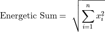
n … Number of CPB bins
xi … CPB bin with index i
In case it is a Decibel spectrum, the calculation is the following:
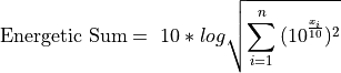
n … Number of CPB bins
xi … CPB bin with index i
If Compute overall Values is enabled, one CPB spectrum averaged for the whole measurement time and an energetic sum (if enabled) averaged for the whole measurement time will be calculated.
The calculation will be reset at recording start. The channel name will be CPB Overall and Energetic Sum Overall (see ④ in Fig. 301).
If Extract individual frequency bands is enabled, frequency bands can be output as time domain channels. I.e. If 100 Hz is entered, the 100 Hz band will be extracted as time domain channel to analyze the time dependent trend.
It is possible to extract several bands (see Fig. 302).
If the entered frequency is not the center frequency of a CPB bin, the bin including this frequency will be extracted.
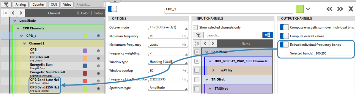
Fig. 302 CPB Analysis with extracted 100 Hz and 250 Hz bin
Array Statistics
To create Array Statistics channels, click the [+] button in the lower left corner of the Data Channels menu (see Working with Software Channels) and select Array Statistics in the* Advanced Mathematics* tab. Before selecting Array Statistics, at least one array channel (e.g., a FFT amplitude channel) must be selected.
The following options are available when creating the array statistics (see Fig. 303):
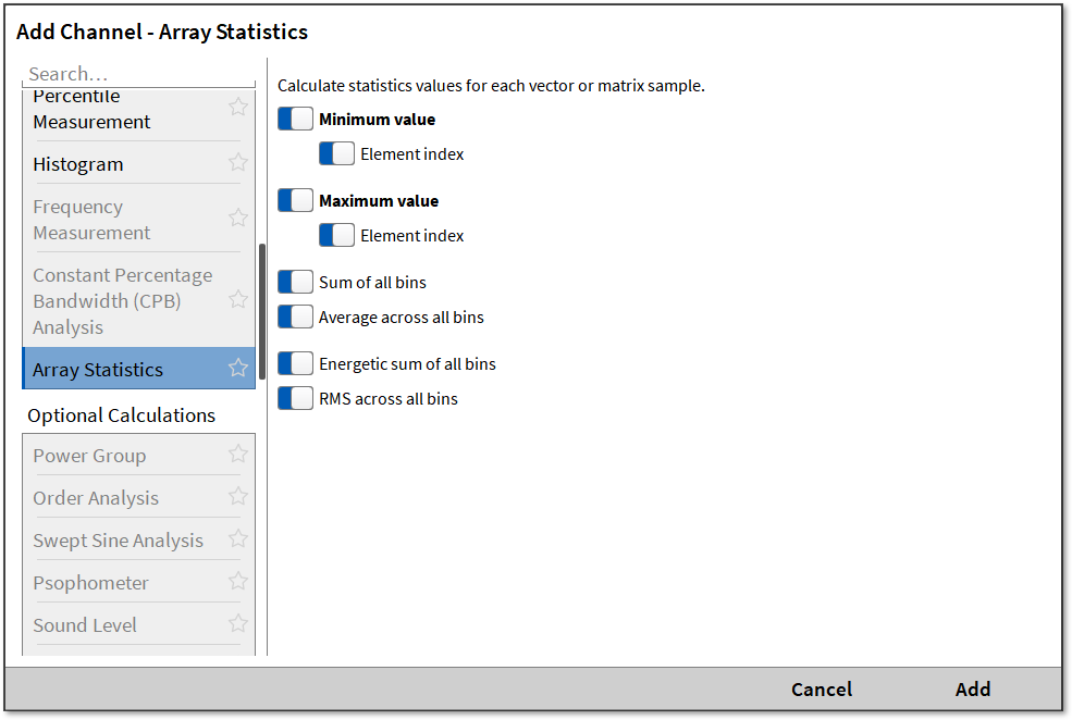
Fig. 303 Options when creating array statistics
Minimum value: Extracts the smallest value from the array
Element index: Extracts the bin and frequency of the smallest value from the array
Maximum value: Extracts the largest value from the array
Element index: Extracts the bin and frequency of the largest value from the array
Sum of all bins: Adds up all bins
Average across all bins: Calculates the linear average from all bins
Energetic sum of all bins: Calculates the quadratic sum from all bins
RMS across all bins: Calculates the RMS from all bins
The selected options each generate a software channel with the respective information for each assigned array channel.
The following figure (Fig. 304) shows an example of the array statistics of an FFT amplitude channel with all options enabled. The update rate of the Array Statistic channels is the same as the underlying array channel, in this case 2 Hz.
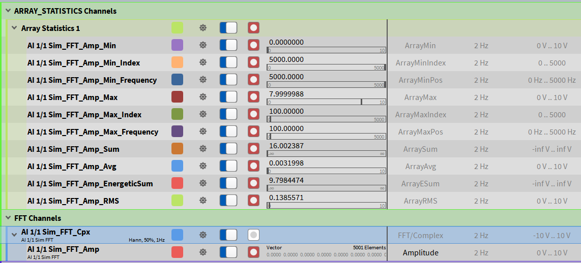
Fig. 304 Example for Array Statistics of a FFT amplitude channel
Difference between Array Statistics and Statistics calculated for array channels
In the add channel window (after pressing “+” in the channel list) there is the Statistics tool in the Basic Math tab and the Array Statistics tool in the Advanced Math tab.
In contrast to Array Statistics, where the selected analysis is performed once over the entire array, creating Statistics for array channels applies the analysis individually to each bin. For example, if an array contains 5001 bins and a maximum statistic is calculated, the resulting statistic channel will contain 5001 maxima — one for each bin. In Array Statistics, however, only a single global maximum across all bins is returned.
The update rate of Array Statistics is fixed to the update rate of the referenced array channel. For Statistics a window size can be selected to adjust the update rate of the statistic. To read more about the Statistics option see the Using Array channels in Statistics chapter.
Optional calculations
Power Group
This is an optional feature and requires a license.
A Power Group can be created by pressing either the Add button or the Calculator button in the lower left corner of the Data Channels menu (both buttons marked red in Fig. 305).
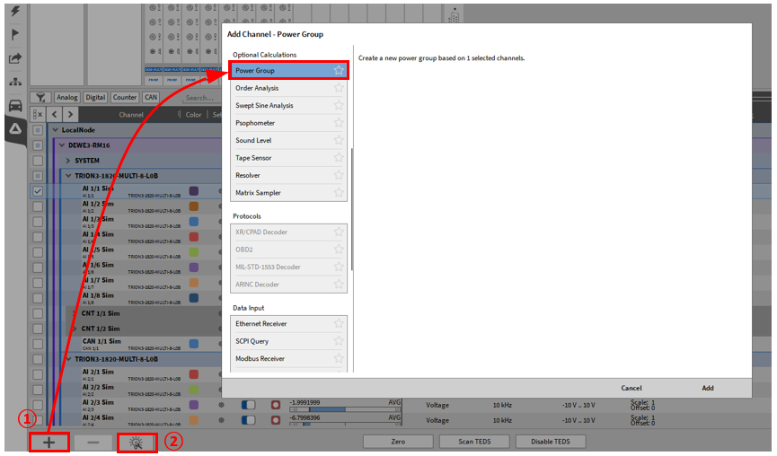
Fig. 305 Pop-up window for creating a Power Group
For more information, refer to the to the OXYGEN Power Technical Reference manual which is available on the DEWETRON CCC-portal (https://ccc.dewetron.com/).
Order Analysis
This is an optional feature and requires a license.
To create an Order Analysis, click the [+] button in the lower left corner of the Data Channels menu (see Working with Software Channels) and select Order Analysis in the Optional Calcualtions tab.
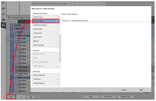
Fig. 306 Pop-up window generating an order analysis
For details about the Order Analysis plugin refer to the DEWETRON_Oxygen_Order_Analysis_vx.x Manual which is available on the DEWETRON CCC-portal (https://ccc.dewetron.com/).
For more information, refer to the to the DEWETRON OXYGEN Order Analysis manual which is available on the DEWETRON CCC-portal (https://ccc.dewetron.com/).
Swept Sine Analysis
This is an optional feature and requires a license.
The Swept Sine Analysis can be used to determine the transfer function and the bode diagram of a DUT that is stimulated by a shaker which is driven by a wave-generator replaying a sine sweep. An exemplary testbed could look like the following (see Fig. 307):
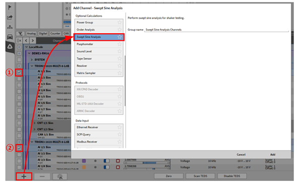
Fig. 307 Exemplary testbed to use the Swept Sine Analysis plugin
A DUT is standing on a shaker. The shaker is driven by a Signal Generator which replays a sine sweep. One accelerometer is applied directly on the shaker and provides the reference (source) signal that is used to stimulate the DUT. One or several additional accelerometers are applied directly on the DUT that measure the acceleration on the DUT surface on different positions (sink).
These signals can be applied to the Swept Sine Analysis plugin to determine the transfer function and the phase shift from source to sink.
Setting up a Swept Sine Analysis
To set up the Swept Sine Analysis plugin, perform the following steps:
At first, mark the checkbox of the channel which provides the reference signal for the Swept Sine Analysis (see ① in Fig. 308)
Next, mark the channel that provides the signal measured on the signal sink (see ② in Fig. 308). Several sink signals could be applied to one Swept Sine Analysis group.
Click on the PLUS (see ③ in Fig. 308) sign to open the math setup and select Swept Sine Analysis. Edit the channel group name if desired and click on the OK button afterwards.
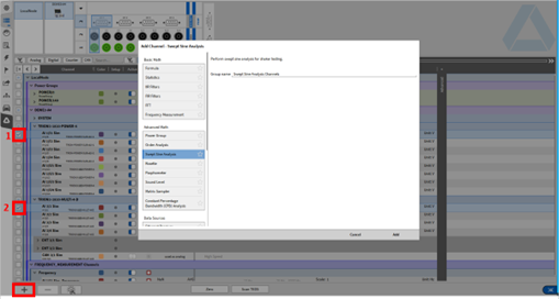
Fig. 308 Swept Sine Analysis
Setup overview
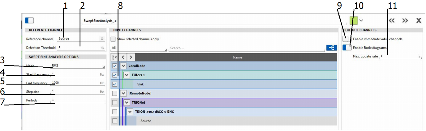
Fig. 309 Swept Sine Analysis setup – overview
No. |
Function |
Description |
|---|---|---|
1 |
Reference channel selection |
The channel that provides the reference signal can be edited here; This channel is used to determine the fundamental frequency which is available in the channel F_fund (see Swept Sine analysis output channels) |
2 |
Detection Threshold selection |
Amplitude threshold for determining the fundamental frequency; If the amplitude of the reference channel is below the specified threshold (percentage of the channel input range), the fundamental frequency will not be determined; I.e. Channel Input Range = 100 V and Detection Threshold = 1%; The signal amplitude must be 1V or higher to determine the fundamental frequency |
3 |
Calculation mode selection |
RMS or Zero-Peak selectable; The output channels (see Swept Sine analysis output channels) may contain either the RMS or Zero-to-Peak level as result |
4 |
Start frequency selection |
Enter the lower frequency limit for the Swept Sine Analysis |
5 |
Stop frequency selection |
Enter the upper frequency limit for the Swept Sine Analysis |
6 |
Step size selection |
Enter the frequency resolution of the Swept Sine Analysis |
7 |
Periods selection |
Number of signal periods of the reference signal that shall be used for updating one value |
8 |
Input channels selection |
Select the input channels that contain the sink signals (sensors that applied on the DUT); One or several sensors can be selected |
9 |
Enable immediate value channels switch |
The channels that contain the time domain signals (see Swept Sine analysis output channels) are enabled with this switch; Per default disabled |
10 |
Enable Bode diagram switch |
The channels that contain the frequency domain signals (see Swept Sine analysis output channels) are enabled with this switch; Per default enabled |
11 |
Max update rate selection |
Select the calculation update rate (from 1 to 10s) |
Swept Sine analysis output channels
F_fund: Contains the fundamental frequency of the Swept Sine Analysis; Calculation based on the signal provided by the reference (source) channel
ChannelName_iRMS or ChannelName_iPeak: Time domain channel; Contains the amplitude (RMS or Zero-to-Peak level depending on the selection in ③ in Fig. 309) of the signal at the actual frequency; The amplitude is only referring to the fundamental frequency signal components; Can be assigned to a Recorder (see Recorder), Digital Meter (see Digital meter) or similar.
ChannelName_iPhi: Time domain channel; Contains the phase shift of the signal at the actual frequency; Can be assigned to a Recorder (see Recorder), Digital Meter (see Digital meter) or similar.
ChannelName_iUFRMS or ChannelName_iUFPeak: Time domain channel; Contains the amplitude (RMS or Zero-to-Peak level depending on the selection in ③ in Fig. 309) of the signal at the actual frequency; The amplitude is referring to the entire signal components; Can be assigned to a Recorder (see Recorder), Digital Meter (see Digital meter) or similar
ChannelName_RMS or ChannelName_Peak: Frequency domain channel; Contains the transfer function (RMS or Zero-to-Peak level depending on the selection in ③ in Fig. 309); The amplitude is referring to the fundamental frequency signal components; Can be assigned to a Spectrum Analyzer (see Spectrum analyzer) instrument for displaying the data.
ChannelName_Phi: Frequency domain channel; Contains the phase diagram; Can be assigned to a Spectrum Analyzer (see Spectrum analyzer) instrument for displaying the data.
ChannelName_UFRMS or ChannelName_UFPeak: Frequency domain channel; Contains the transfer function (RMS or Zero-to-Peak level depending on the selection in ③ in Fig. 309); The amplitude is referring to the entire signal components; Can be assigned to a Spectrum Analyzer (see Spectrum analyzer) instrument for displaying the data.
Calculation remarks
The maximum frequency span is from 1 to 20000 Hz. To achieve a suitable accuracy, it is recommended to set the sample rate of the input channels to at least 20 times the maximum frequency, i.e. to 20 kHz in case of 1 kHz maximum frequency span.
The highest resolution of the frequency domain channels is 1 Hz. Data of non-integer frequency bins is rounded to the next integer frequency bin.
If the sweep does not exactly hit exactly one frequency bin which is contained in the data array, data for the certain frequency bin is filled up by linear interpolation of the two narrowed frequency bins
The channels containing frequency domain data contain only one single value data array at the end of the measurement. In case of multi-file recording (see Multi-file recording), this data array will only be included in the last data file, the other files will not contain this data.
If the sweep is passing the same frequency several times, there will not be several values for the same frequency stored, but the maximum value only is stored to the data file.
If the screen is frozen (see ⑦ in Fig. 14) and the orange cursor is moved either in the Overview Bar or in a Recorder, the data of the single value array will change approximately every second as the array is continuously filled with data. In the end, there will only be the final value.
As the channels containing frequency domain data contain only one single value data array at the end of the measurement, there will not be reduced Statistics data available (see Triggered Events).
Psophometer
In telecommunications, a psophometer is an instrument that measures the perceptible noise of a telephone circuit.
The core of the meter is based on a true RMS voltmeter, which measures the level of the noise signal. This was used for the first psophometers, in the 1930s. As the human-perceived level of noise is more important for telephony than their raw voltage, a modern psophometer incorporates a weighting network to represent this perception. The characteristics of the weighting network depend on the type of circuit under investigation, such as whether the circuit is used to normal speech standards (300 Hz – 3.3 kHz), or for high-fidelity broadcast-quality sound (50 Hz – 15 kHz).
Setup
The Psophometer plugin is installed with every OXYGEN installation, starting from R3.5.1
A dedicated plugin license is required for the calculation option to be visible.
Usage
Select one or multiple channels as inputs for the Psophometer calculation.
Note
Input channels must have a sampling rate of 20 kHz or higher.
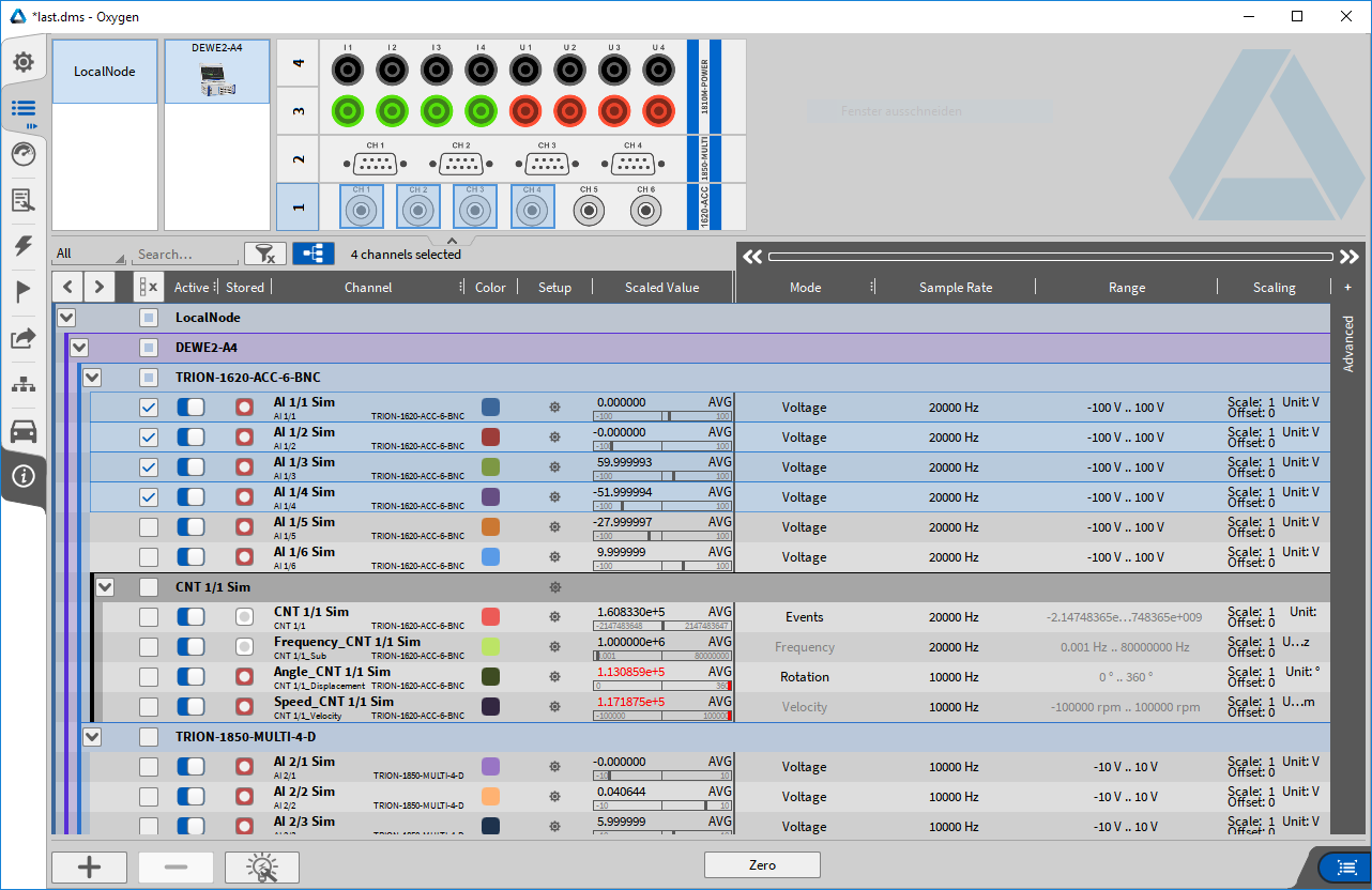
Fig. 310 Channel list with multiple selected channels
Then open the “Add Channel” dialog by pressing the plus button.
Select Psophometer. The dialog now shows the Psophometer frequency weighting settings (see Weighting) which can be made.
The newly created Psophometer calculation group can be named individually.
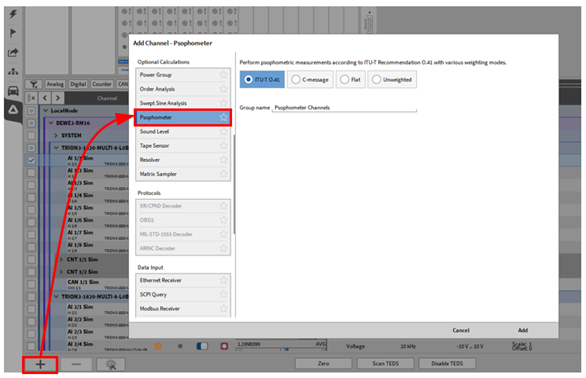
Fig. 311 Add Channel dialog showing Psophometer options
Finally, press Add to create the new calculation group.
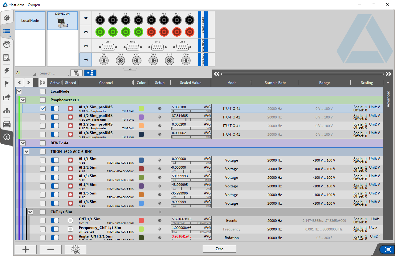
Fig. 312 Channel list showing new Psophometer calculation group
The channel setup is used to modify each channel’s settings and a top review of signals. Additionally, depending on the selected mode, connector pinout is displayed.
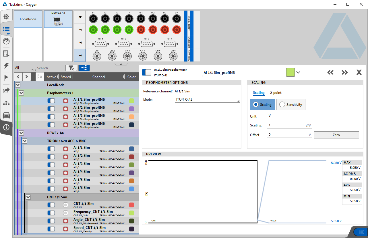
Fig. 313 Channel setup, preview, and pin out and connection
Psophometer calculations are then available as math channels.
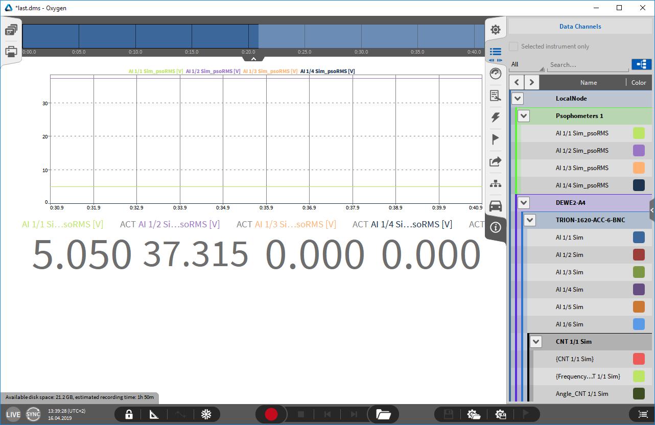
Fig. 314 Sidebar channel list showing the calculated Psophometer channels
Calculation
The calculation is based on FFT.
Depending on the input sampling rate, the FFT block size is chosen to be 2^N samples while the time window stays between 75 and 125 ms, to ensure passing the detector circuitry tests (see ITU-T Recommendation O.41 (10/94)).
Sampling rate |
FFT block size |
|---|---|
20 kHz |
2048 |
50 kHz |
4096 |
100 kHz |
8192 |
200 kHz |
16384 |
Weighting
Different weighting options are available:
ITU-T O.41
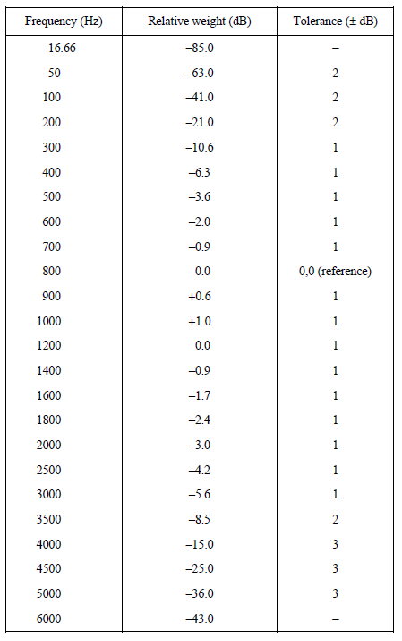
Fig. 315 Telephone circuit Psophometer weighting coefficients and limits
C-message
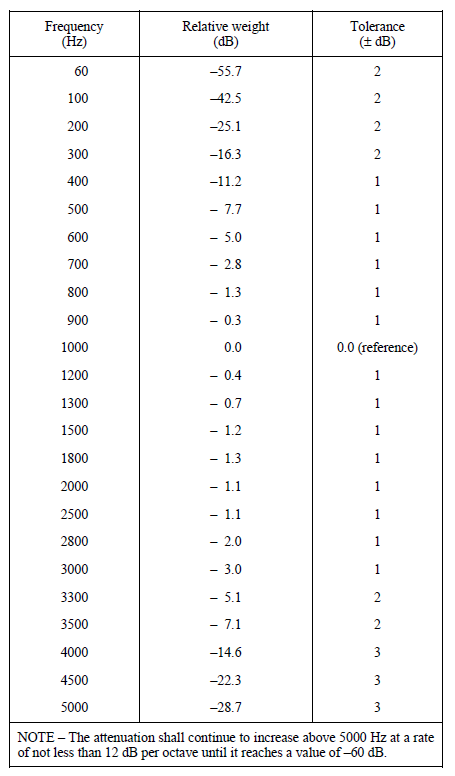
Fig. 316 C-message weighting coefficients and accuracy limits
Flat
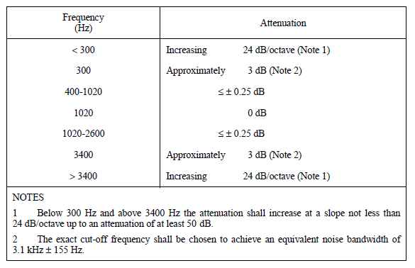
Fig. 317 Characteristics of the optional flat filter with an equivalent noise bandwidth of 3.1 kHz (bandwidth of a telephone channel)
Unweighted
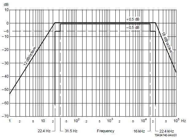
Fig. 318 Frequency response characteristics for unweighted measurements
Comparison between Psophometric and C-message weighting
Fig. 319 Comparison between psophometric and C-message weighting
ITU-T Recommendation O.41 (10/94)
OXYGEN Sound Level plugin
This is an optional feature and requires a license.
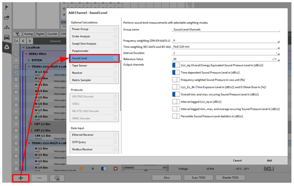
Fig. 320 Pop-up window for generating a sound level plugin
A Sound Level can be created and configured by pressing the Add button in the lower left corner of the Data Channels menu (marked red in Fig. 320).
For more information, refer to the to the DEWETRON Sound Level determination manual which is available on the DEWETRON CCC-portal (https://ccc.dewetron.com/).
Modal test
This is an optional feature and requires a license (OXY-OPT-MODAL).
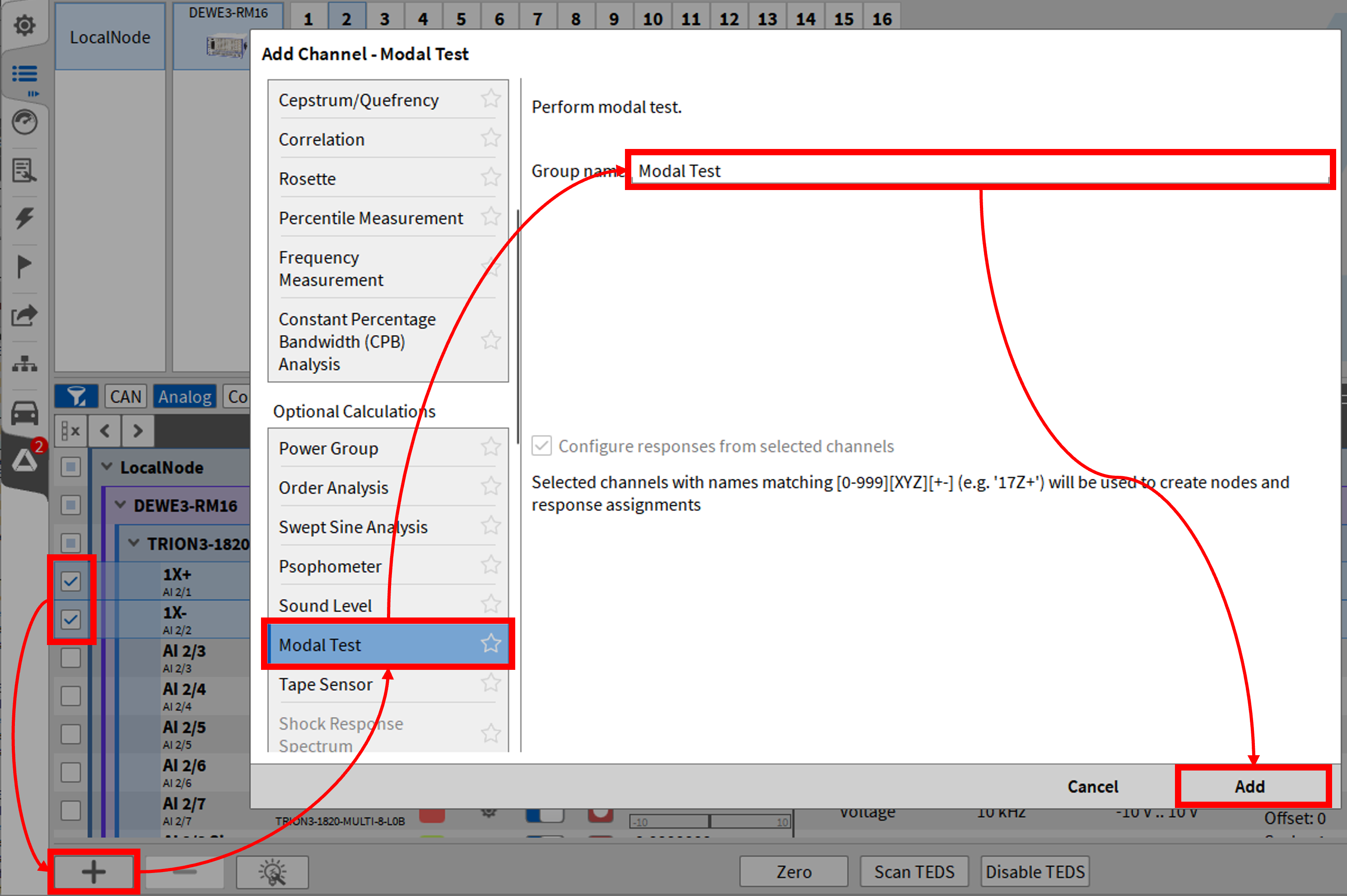
Fig. 321 Pop-up window for generating a Modal Test plugin
A Modal Test can be created in LIVE mode and configured by pressing the Add button in the lower left corner of the channel list (marked red in Fig. 321).
For more information, refer to the to the DEWETRON OXYGEN Modal Technical Reference manual which is available on the DEWETRON CCC-portal (https://ccc.dewetron.com/).
Tape Sensor
This is an optional feature and requires a license (OPT-TAPE-RES).
OXYGENs Tape Sensor and Resolver Plugin allows speed and angle determination for Tape Sensors (black and white striped band with optical sensor) and for Resolvers with and without envelope detection.
For more information, refer to the to the OXYGEN Tape Sensor und Resolver Manual manual which is available on the DEWETRON CCC-portal (https://ccc.dewetron.com/).
Resolver
This is an optional feature and requires a license (OPT-TAPE-RES).
OXYGENs Tape Sensor and Resolver Plugin allows speed and angle determination for Tape Sensors (black and white striped band with optical sensor) and for Resolvers with and without envelope detection.
For more information, refer to the to the OXYGEN Tape Sensor und Resolver Manual manual which is available on the DEWETRON CCC-portal (https://ccc.dewetron.com/).
Shock Response Spectrum
This is an optional feature and requires a license (OXY-OPT-SRS).
The Shock Response Spectrum helps to understand how different systems react to sudden movements or impacts. It is used to calculate the maximum movement of structures and to create requirements for the design of buildings or machines that must withstand sudden loads, such as earthquakes or explosions.
An acceleration signal is applied to a series of mass-damping systems for defined frequency sections, the deflection is determined in maximum, minimum or absolute maximum and entered in a diagram for the respective frequency.
The following figure Fig. 322 shows the calculation process. The acceleration input can be seen at the bottom right as a half-sine, which is broken down into its spectral components and applied to single-degree-of-freedom (SDOF) oscillating elements. The response, i.e. the SDOF acceleration response, is then analyzed for the maximum in the example and plotted in the shock response spectrum above. The oscillating elements are defined solely by their damping factor, hence Single-Degree-Of-Freedom.
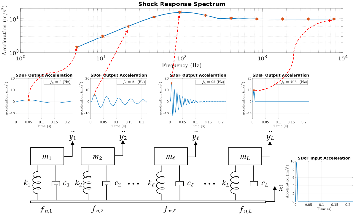
Fig. 322 Schematic procedure for calculating a shock response spectrum
[06.05.2025 https://de.mathworks.com/help/signal/ug/practical-introduction-to-shock-waveform-and-shock-response-spectrum.html]
A Shock Response Spectrum (SRS) can be configured in PLAY mode (*.dmd) by selecting at least one input channel and pressing the Add button in the lower left corner of the channel list (marked red in Fig. 323). If the Group name is left empty, the group is named “SRS_n” by default (n=1,2,3).
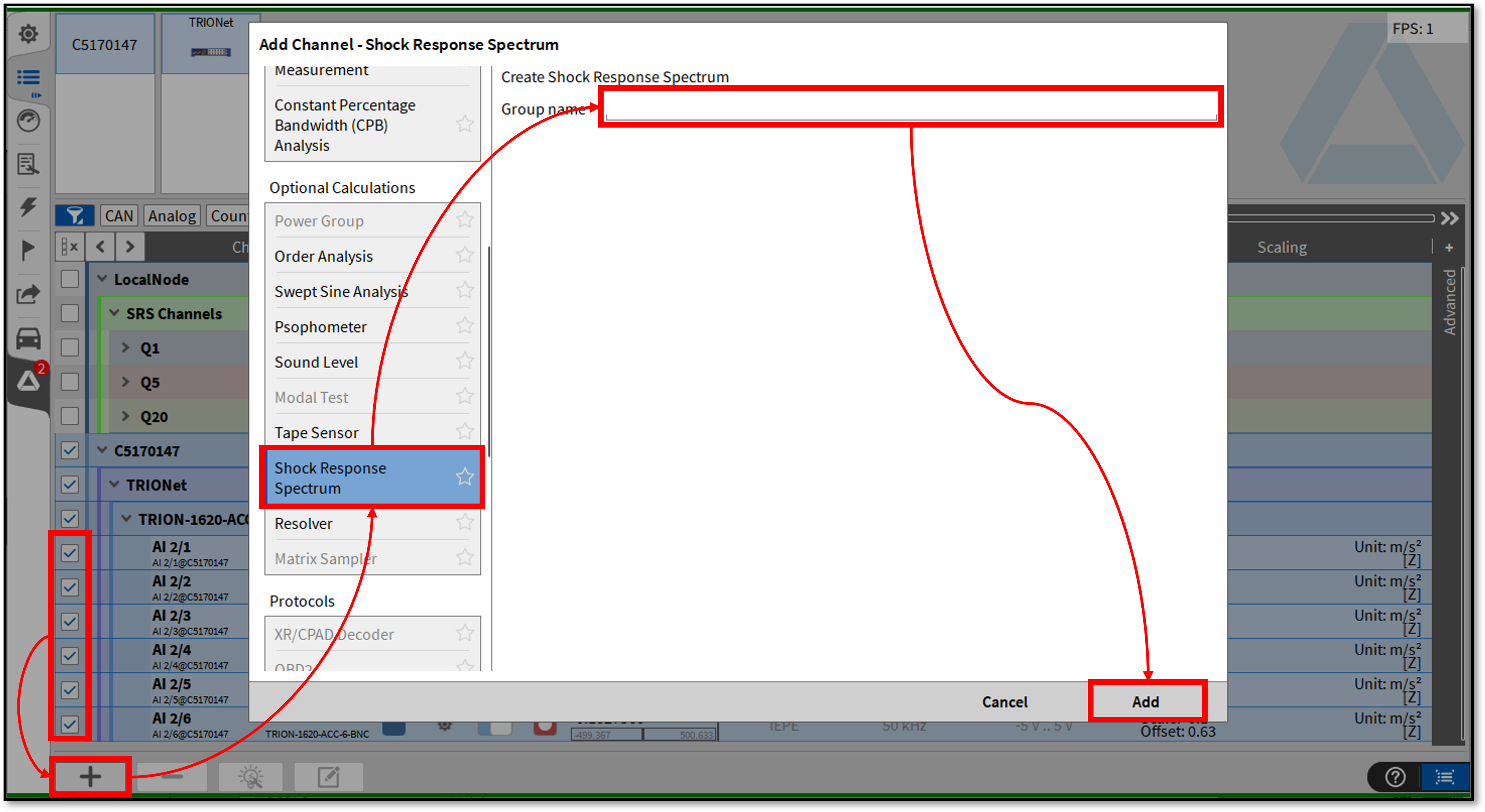
Fig. 323 Pop-up window for generating Shock Response Spectrum plugin
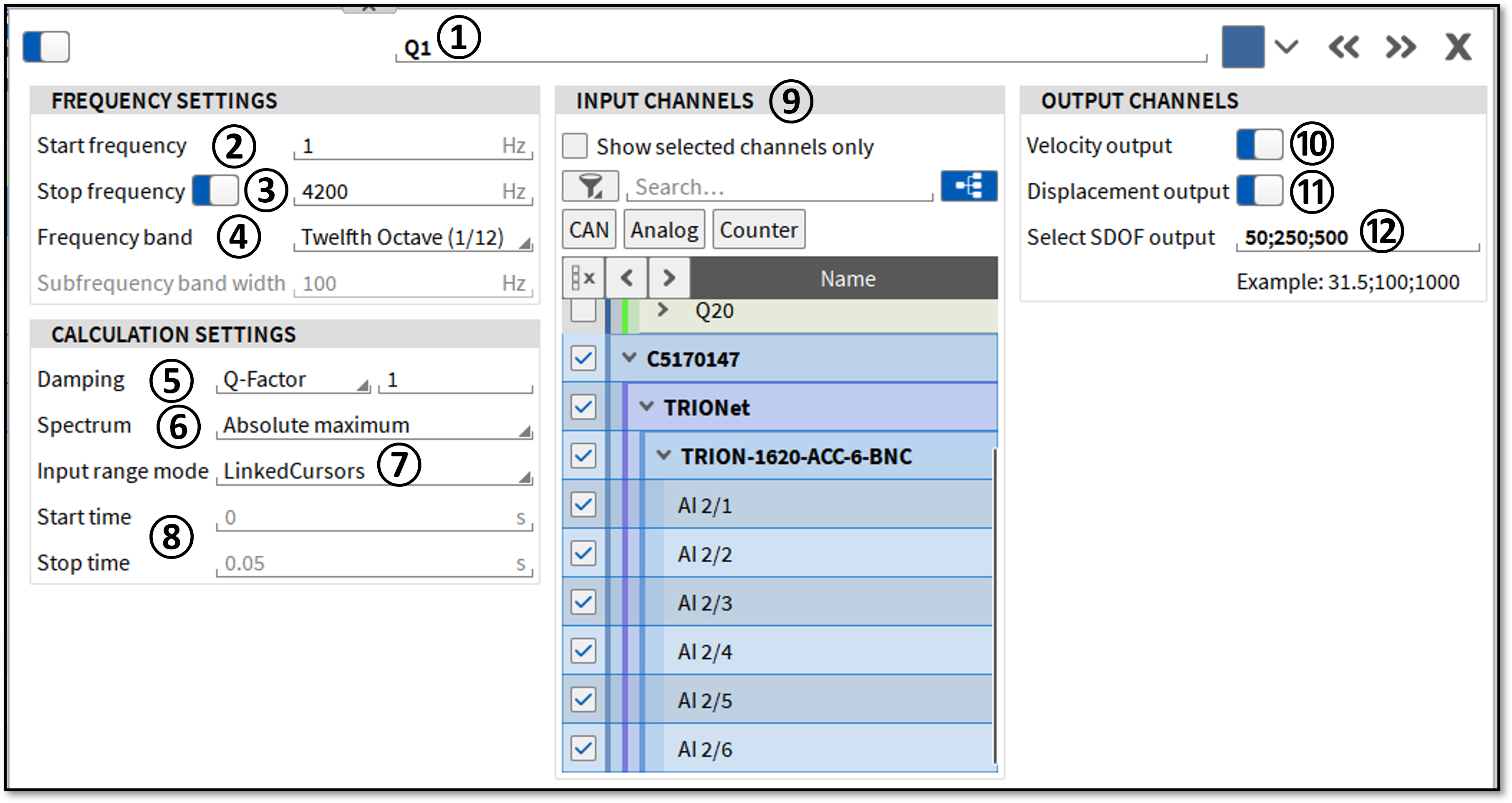
Fig. 324 Setup of Shock Response Spectrum plugin with calculation setting
Index |
Name |
Description |
|---|---|---|
1 |
SRS channel group name, by default SRS_n (n=1,2,3) |
Set the name of the shock response spectrum channel group, which always includes the acceleration shock response. |
2 |
Start frequency |
Define the starting frequency for the shock response spectrum calculation. Valid values are (0.01 Hz up to the stop frequency) |
3 |
Stop frequency |
Define the end frequency of the shock response calculation. With the toggle automatically half the sample rate as stop frequency is set. Valid values are (Start frequency up to half the sample rate) |
4 |
Frequency band |
Select the frequency band in which the SRS is calculated. If “Linear” is selected, the subfrequency band width text field below is enabled. For octave bands the octave, 1/3 octave and 1/12 octave band are available. |
5 |
Damping |
Define the damping via Q-factor or damping ratio by choosing the respective dropdown option and value. |
6 |
Spectrum |
Select either one spectrum of the single degree of freedom (SDOF) elements, Absolute maximum, Maximum or Minimum. |
7 |
Input range mode |
Define the time frame selection method. In case “Manual” is selected, the Start time and Stop time in point ⑧ are used for calculation. |
8 |
Start/Stop time |
In case the input range mode is set to “Manual” the time frame for SRS calculation is done for the samples between start and stop time. |
9 |
Input channels |
List view of channels for whom the SRS is calculated. These channels can be changed anytime, but their sample rate must be equal. Expected input channels are acceleration channels in m/s2. |
10 |
Velocity output |
Additional to the SRS of acceleration, the time integral of the acceleration, the velocity can be enabled. |
11 |
Displacement output |
Additional to the SRS of acceleration, the second time integral of the acceleration, the displacement can be enabled. |
12 |
Select SDOF output |
Define for which frequencies the SDOF acceleration elements should be added to the SRS group. If the input frequency is not the center frequency of the SDOF element, the closest element is chosen. |
To link AB-cursor as the timeframe for the SRS calculation of any SRS group, enable AB-cursor and click on the button to the right to the AB-cursor checkbox, select the SRS groups that should be linked to the cursor and click Ok. Moving the cursor now changes the timeframe for which the SRS is calculated.
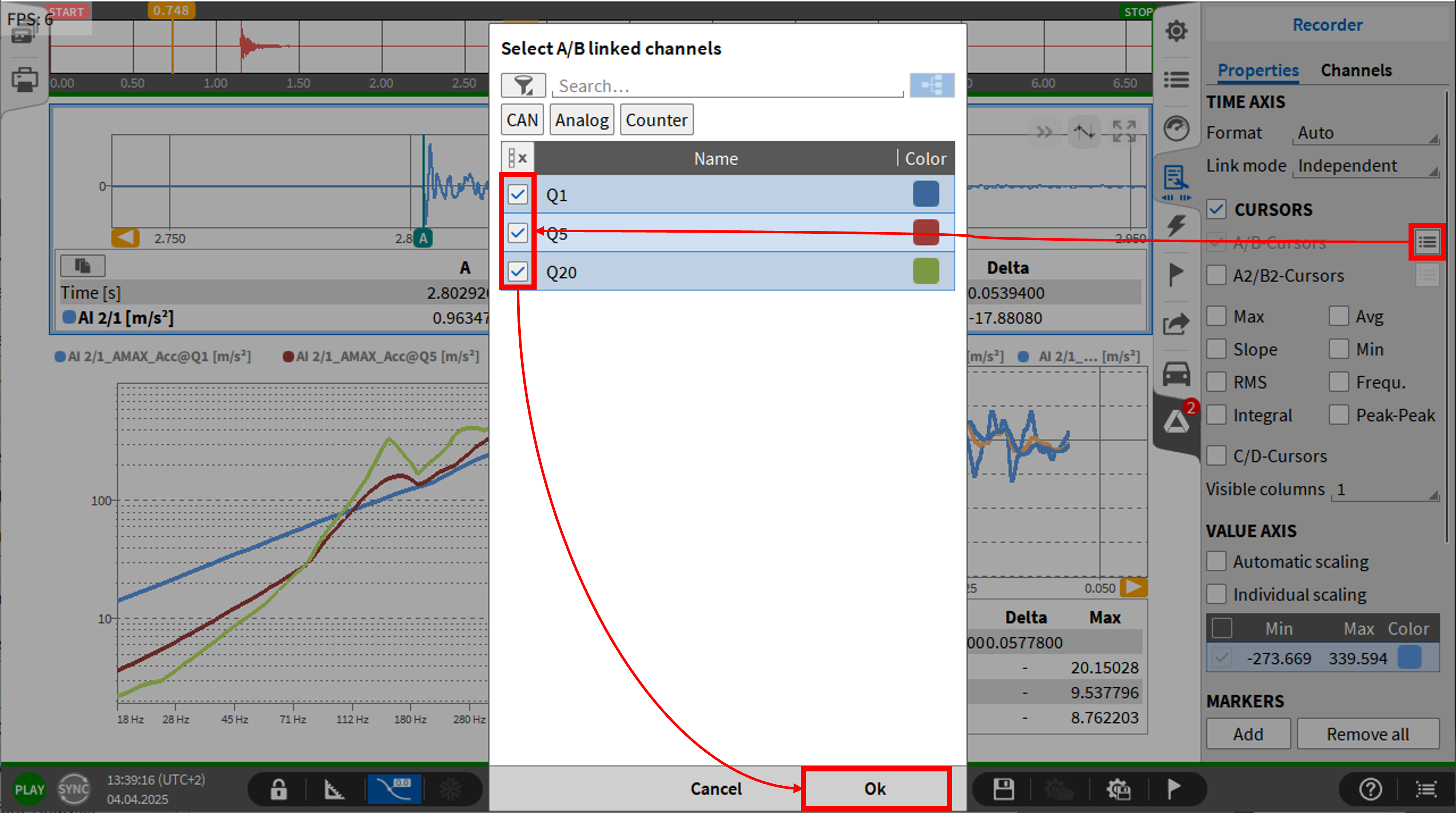
Fig. 325 Link AB-cursor as timeframe for SRS calculation
The SRS channels (acceleration, velocity, and displacement) are 1D arrays. For example, e.g. “AI 2/1_AMAX_Acc” has one acceleration per bin/frequency and can be displayed in an Array chart. The array chart can be copied and pasted for further analysis. The extracted SDOF channels are the acceleration-time response of the damping elements for the selected frequencies and can be displayed in a recorder.
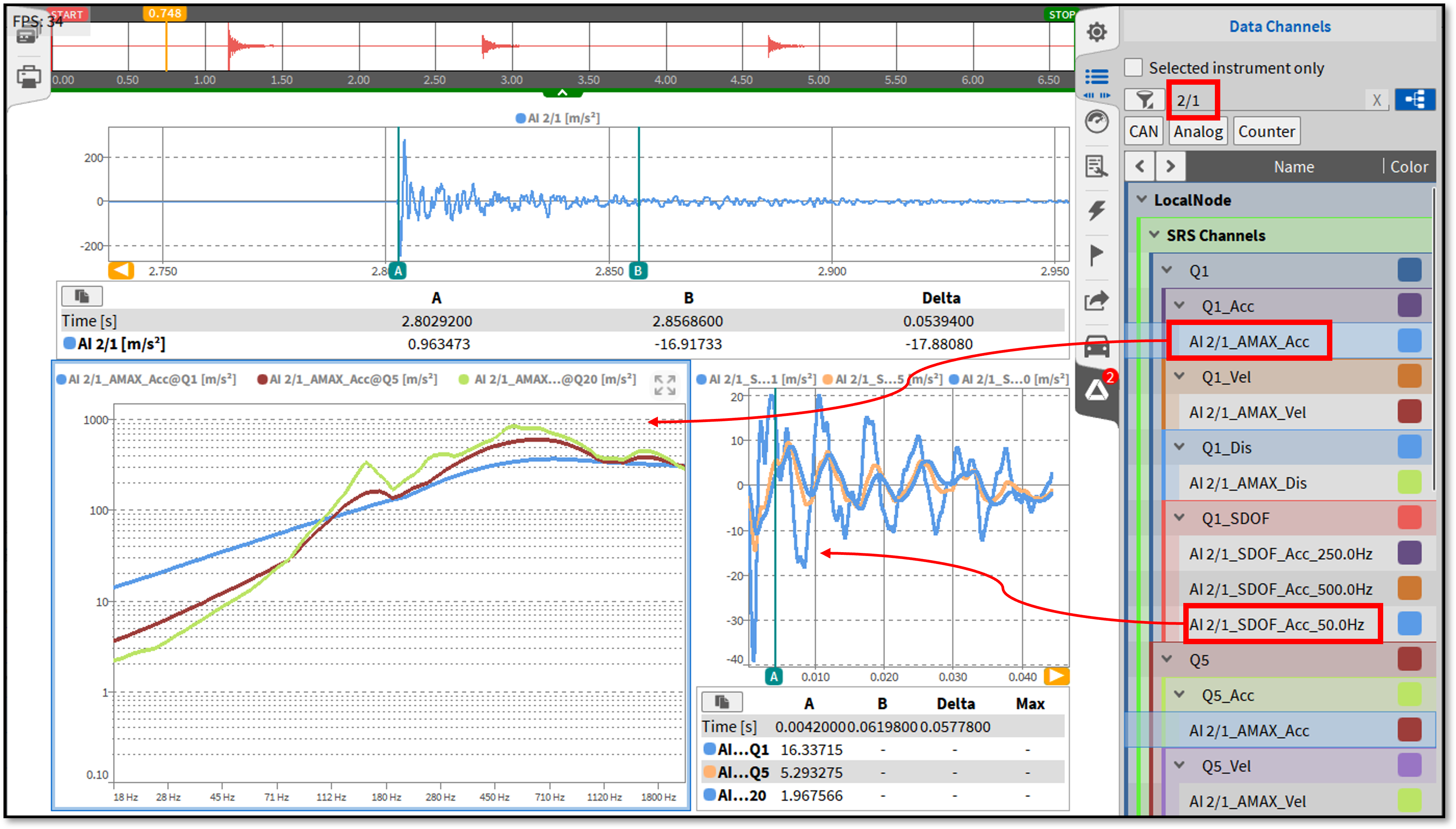
Fig. 326 Show SRS data in instruments
Note
Note that to update the time interval in the calculation the Edit Mode must be active. This is done in the channel list with the Edit already stored channels button.
Matrix Sampler
This is an optional feature and requires a license (OPT-POWER-ADV).
The matrix sampler is a feature, which is included in the advanced Power calculation. This feature displays the relation between two channels and an input channel in form of a color-coded matrix which is displayed in the Intensity Diagram instrument.
Creation of a Matrix Sampler Channel
There are two ways to create a matrix sampler channel:
Click the [+] button in the lower left corner of the Data Channels menu (see Working with Software Channels) and select Matrix Sampler in the Optional Calculations tab. Before selecting Array Statistics, at least one array channel (e.g., a FFT amplitude channel) must be selected. The desired reference channels can be selected in advance or selected afterwards.
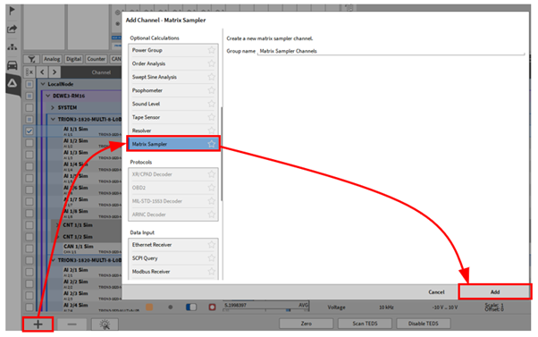
Fig. 327 Creation of a Matrix Sampler channel from channels in the channel list
The other possibility to create a matrix sampler channel in form of an efficiency map is in the Power Group settings. For a detailed explanation on how to create a Power Group see Power Group refer to the to the OXYGEN Power Technical Reference manual which is available on the DEWETRON CCC-portal (https://ccc.dewetron.com/).
Open the Power Group settings and go to Efficiency in the advanced settings. By simply clicking on the Add efficiency map button (see Fig. 328), a matrix sampler channel will be created with the according channels (speed, torque, and efficiency) to display the respective efficiency map of the Power Group.
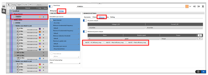
Fig. 328 Creation of a Matrix Sampler channel as an efficiency map of an according Power Group
After creating a matrix sampler channel by either one of these ways, a new section appears in the channel list seen in Fig. 329. For each matrix sampler one new channel will be created.

Fig. 329 New section for Matrix Sampler channels in the channel list
Matrix Sampler Channel Settings
Some of the channel settings of the matrix sampler channel in this section will be explained by the example of an efficiency map. However, the settings or channels are not bound to a unit of a channel and can be used with any measured channel. An overview of the channel settings can be seen in Fig. 330. To enter the channel settings, click on the gear icon of the channel in the channel list (see Fig. 329).
The following section will explain all the settings, respectively.
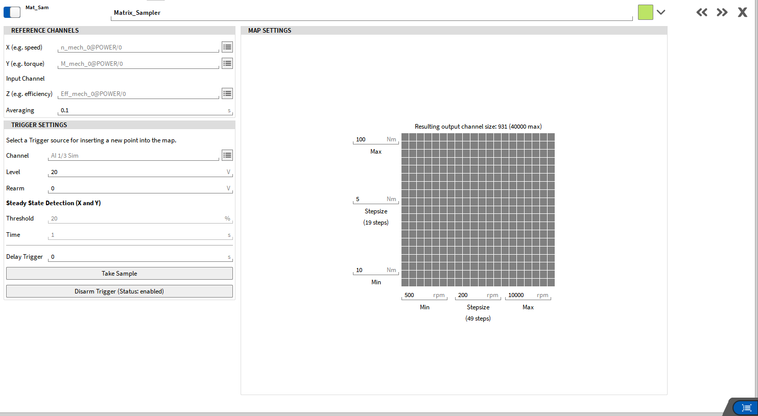
Fig. 330 Channel settings of a Matrix Sampler channel
Fig. 331 shows a detailed overview of the available channel settings of a matrix sampler channel.
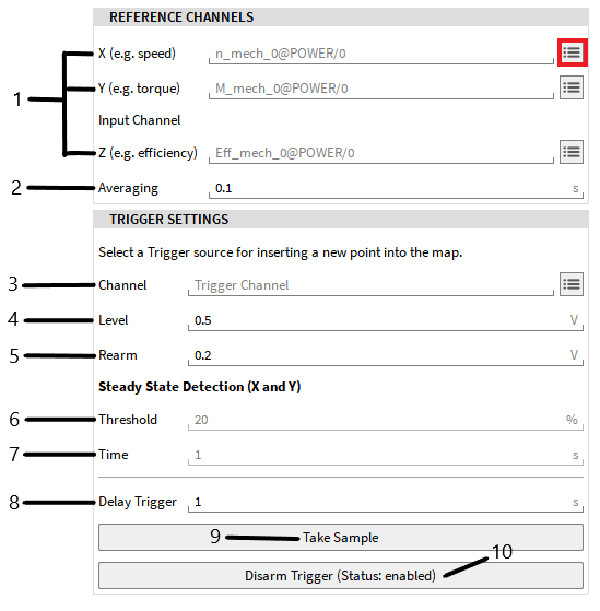
Fig. 331 Detailed view of the setting of a Matrix Sampler channel
No. |
Function |
Description |
|---|---|---|
1 |
X, Y, Z reference channels selection |
The reference channels for X, Y and Z can be selected here. Z acts as the input channel, which will be displayed. Channels can also be assigned via drag’n’drop or by clicking on the channel list button marked in red in Fig. 331 |
2 |
Averaging |
The time window to calculate the average of input channel Z |
3 |
Trigger Channel |
Selection of a trigger channel; this channel is used as a trigger to take a sample for the matrix |
4 |
Trigger Level |
Defines the level upon which the trigger is initiated |
5 |
Rearm |
Defines the rearm level, upon which the trigger will be reactivated |
6 |
Threshold |
Defines the range within the X and Y signal must stay in order to arm the trigger |
7 |
Time |
Defines the time of the X and Y signal to stay within the defined threshold range to arm the trigger |
8 |
Delay Trigger |
Defines the time delay, after which a sample will be put into the matrix after the trigger is activated |
9 |
Take Sample |
Button to manually take a sample to put in the matrix |
10 |
Disarm/Arm Trigger |
Trigger settings will be disarmed/armed; if disarmed matrix will not be updated anymore |
As explained in the section before, the channels can either be chosen in the right order before creating the matrix sampler channel, but they can also be changed or assigned via drag’n’drop or the channel list button afterwards.
The channels for an efficiency map are assigned properly when creating an efficiency map out of the Power Group settings. For an efficiency map the speed is used as the reference channel for the X-axis, torque for the Y-axis and the mechanical efficiency for the Z-axis as input channel.
For the trigger channel a signal can be used from a testbed environment to define, when a sample should be put into the matrix. In the example shown in Fig. 331 it can be seen, that a sample will be taken whenever the channel Trigger Channel rises above a defined level of 0.5 V. The trigger will be activated again, once the Trigger Channel drops below 0.2 V, which is defined as the rearm level.
Note
For the trigger settings, either a channel can be selected as trigger or the Steady State Detection (X and Y) can be used. If a channel is selected as trigger channel, the Steady State Detection is disabled. To use the Steady State Detection no channel can be selected as trigger channel or must be deleted. The conditions threshold and time for the Steady State Detection have to be fulfilled by the X and the Y channel in order to arm the trigger.
The Disarm/Arm Trigger button is very useful if a specific measurement point needs to be repeated. In order not to overwrite the whole matrix, the trigger can be disarmed. Therefore, the matrix will not be updated for each trigger, and samples are not saved. Whenever the measurement point is reached, a sample can manually be put in the matrix by clicking the Take Sample button.
Fig. 332 shows the exemplary resulting output matrix in the channel settings. For each the Y- and the X-axis the minimum, maximum and step size can be defined in the corresponding channel unit. When entering the step size, the resulting steps are displayed below.
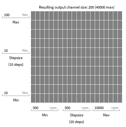
Fig. 332 Detailed view of the map setting of a Matrix Sampler channel
To display this efficiency map on the measurement screen simply drag and drop the matrix sampler channel onto the measurement screen. Otherwise use the intensity diagram instrument and select the channel accordingly.
For more information about the instrument refer to Intensity Diagram.
Protocols
MIL-STD-1553 Decoder
For details about the MIL-STD-1553 Decoder plugin refer to the MIL-STD-1553 Decoder manual which is available on the DEWETRON CCC portal.
ARINC Decoder
For details about the ARINC Decoder plugin refer to the ARINC Decoder manual which is available on the DEWETRON CCC portal.
Data input
OXYGEN Ethernet Receiver
This is an optional feature and requires a license.
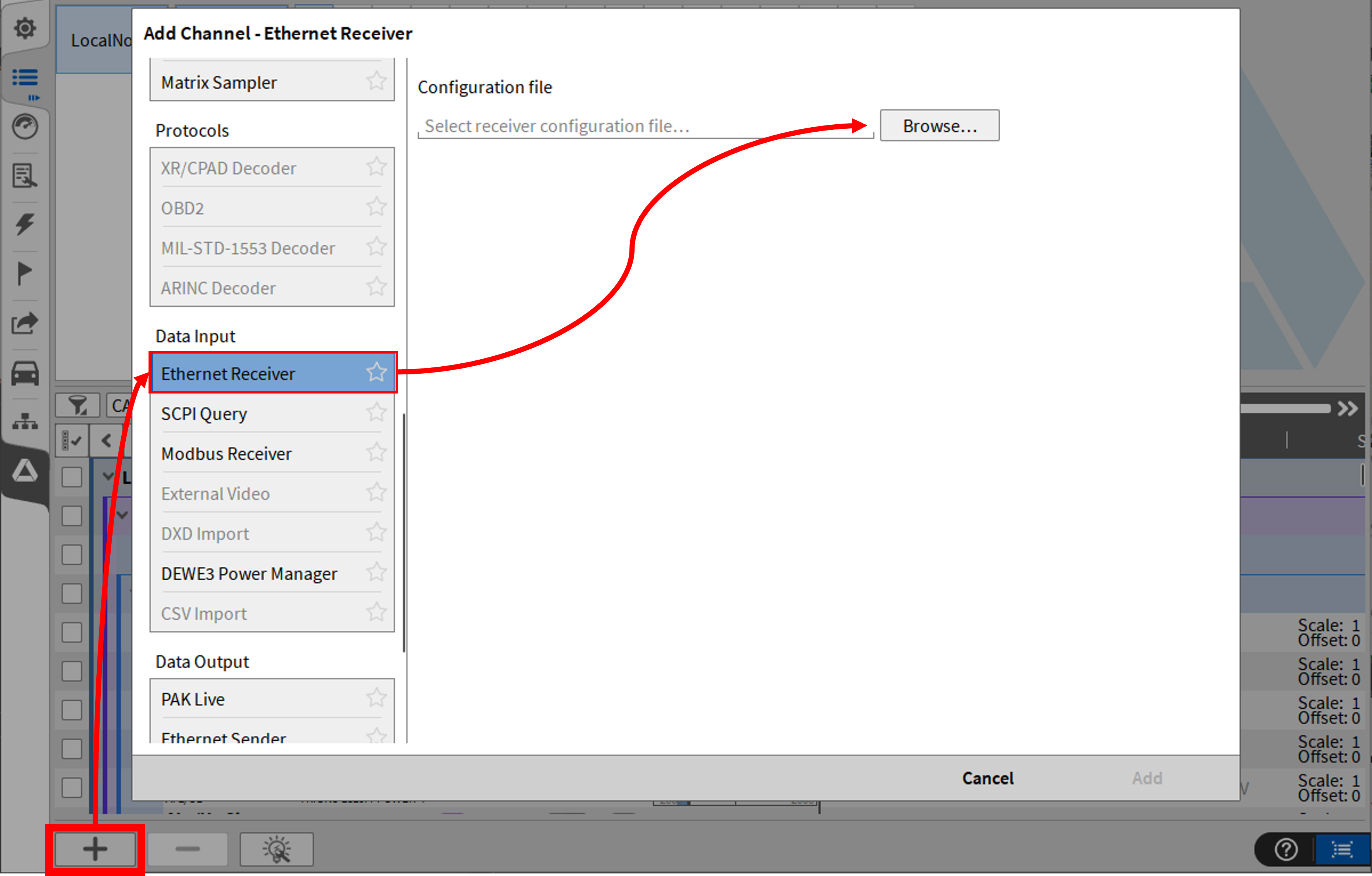
Fig. 333 Pop-up window for acquiring an Ethernet Receiver Data stream
An Ethernet Receiver data stream can be acquired and configured by pressing the Add button in the lower left corner of the Data Channels menu (marked red in Fig. 333).
For details about the Ethernet Receiver plugin refer to the OXYGEN Ethernet Receiver XML Configuration manual which is available on the DEWETRON CCC portal.
SCPI Query
This feature facilitates OXYGEN to fetch data from SCPI compatible devices.
For details about the Ethernet Receiver plugin refer to the OXYGEN SCPI Query manual which is available on the DEWETRON CCC portal.
OPC UA Client
OXYGEN offers an integrated OPC UA Client plugin that allows to subscribe data from OPC UA Servers with a sampling interval up to 1 ms.
For more information, refer to the to the OXYGEN OPC UA Technical Reference Manual which is available on the DEWETRON CCC-portal (https://ccc.dewetron.com/).
Modbus Receiver
This feature facilitates OXYGEN to use Modbus devices as data sources.
For details about the Modbus receiver plugin refer to the OXYGEN Modbus TCP manual which is available on the DEWETRON CCC portal.
External video
The External Video tool imports videos into OXYGEN measurement files (.dmd).
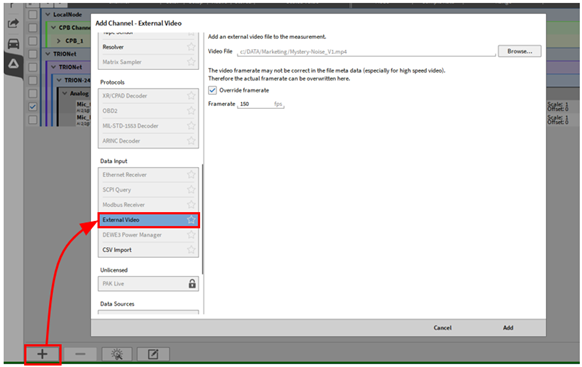
Fig. 334 Pop-up window for loading an external video
OXYGEN’s External video () option provides the possibility to:
Load an video file that was recorded with a 3rd party software in PLAY mode during analysis
Manually synchronize the video to the measurement data
Analyze both video and sensor data synchronized in OXYGEN
This feature was mainly developed to synchronize video data recorded with highspeed cameras to the sensor data but it can be used to load a video file from any camera into OXYGEN. The focus of the following section is on high speed video data.
Benefits:
Load videos from any camera into OXYGEN for analysis
Supported formats:
AVI (uncompressed)
MKV (VP8 and h264)
MP4 (h264)
No file size increment as only path to video file is stored to the .dmd-file
Support of various recording and trigger scenarios (see Possible Recording scenarios)
Adjustable playback speed (see Reviewing a Data File (PLAY mode))
Quick and easy reporting by exporting measurement screen to video (see Saving the screen as video)
Possible Recording scenarios
The section describes different scenarios to initiate the recording start of the DAQ system and the camera and lists certain advantages or disadvantages of the different methods.
Recording start of DAQ system and camera triggered by external signal
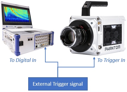
Fig. 335 Recording start of DAQ system and camera triggered by external signal
An external signal / device is used to trigger the recording start of DAQ system and camera. The signal is normally a TTL signal with a rising edge to initiate the recording start.
Modern highspeed cameras provide trigger signal input. The DAQ system requires a digital signal input to acquire the signal and trigger the recording state. Analog inputs could be used as well.
Advantages:
Parallel recording start of camera and DAQ system without any latencies
Easy synchronization of sensor data and video data
No manual recording start on any device required
Disadvantage:
Separate hardware required for generating the trigger signal
Recording start of DAQ system triggered by camera
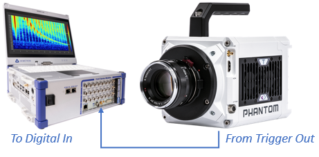
Fig. 336 Recording start of DAQ system triggered by camera
The camera generates a TTL signal with rising edge at recording start which is forwarded to the DAQ system via the Trigger output of the camera. Modern highspeed cameras provide a trigger signal for triggering the recording state of 3rd party hardware. The DAQ system requires a digital signal input for acquiring the signal and triggering the recording state. Analog inputs could be used as well.
Advantages:
Parallel recording start of camera and DAQ system without any latencies
Easy synchronization of sensor data and video data
No separate hardware required for generating the trigger signal
Disadvantage:
Recording must be started manually for the camera
Recording start of camera triggered by DAQ system
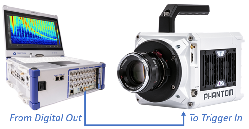
Fig. 337 Recording start of camera triggered by DAQ system
The DAQ system generates a TTL signal with Rising edge at recording start which is forwarded to the camera via an digital output of the DAQ system. Modern highspeed cameras provide a trigger signal input.
The operating system of the DAQ system will cause a delay between the DAQ system’s recording start and the instant of time the digital output is physically set to high which results in the recording start of the camera. This delay can be measured by recording the Digital Out channel. In real-life, a delay in the msec-range between DAQ system recording start and camera recording start will occur which can be compensated while loading the video into OXYGEN for post processing.
Advantages:
No separate hardware required for generating the trigger signal
Recording start of the DAQ system could be triggered
Disadvantages:
Deterministic latency between recording start of camera and DAQ system caused by the operating system
Latency needs to be compensated while loading and post processing the video
Manual Recording start of DAQ system and camera
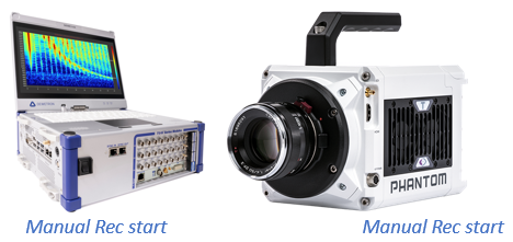
Fig. 338 Manual Recording start of DAQ system and camera
Recording is started manually both on the DAQ system and the camera.
Advantages
No separate hardware required for generating the trigger signal
No wiring between camera and DAQ system required
Disadvantages
Stochastic latency between recording start of camera and DAQ system caused by the operating system
Latency needs to be determined empirically and compensated while loading and post processing the video
Loading the external video into OXYGEN
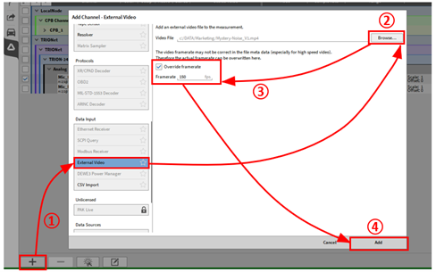
Fig. 339 Procedure to load an external video
To load an external video proceed the following steps:
Synchronization of external videos
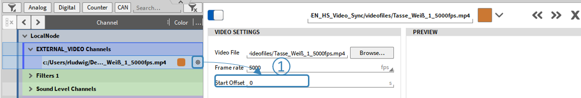
Fig. 340 Compensating a deterministic delay between video and sensor data
If the latency between video and sensor data is known it can be compensated by entering the delay in Start Offset in the video’s channel setup (see ① in Fig. 340).
Positive offset denotes that OXYGEN data recording was started first and video data recording second.
Negative offset denotes that video data recording was started first and OXYGEN data recording second.
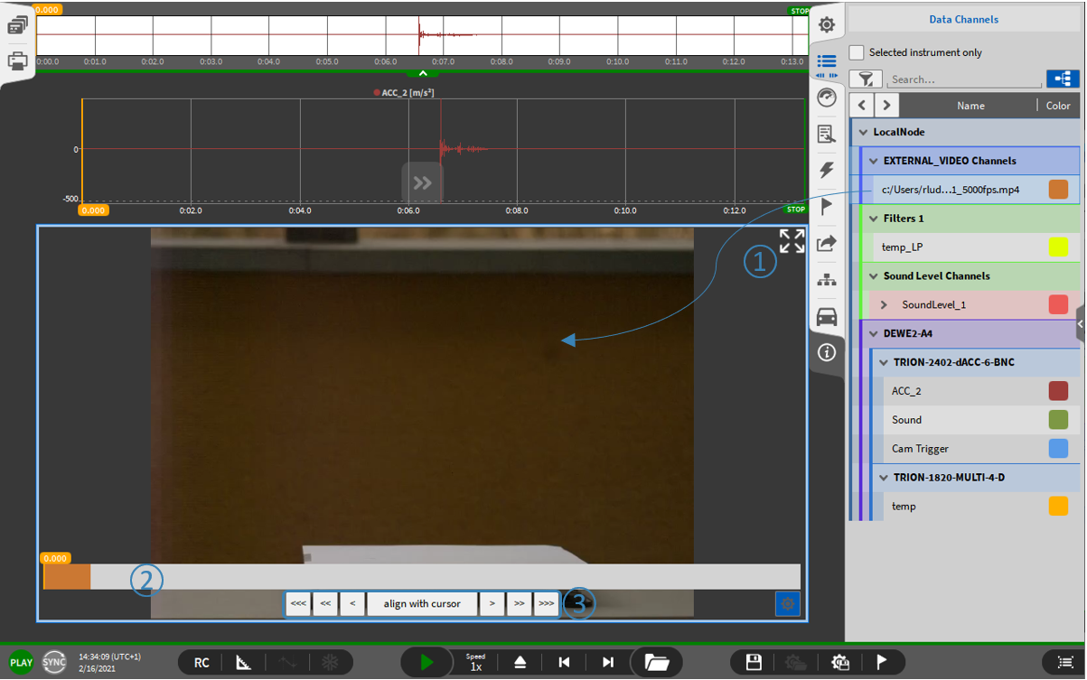
Fig. 341 Manual delay compensation between video and sensor data
If the latency between video and sensor data in unknown, the video timeline can be aligned to sensor data’s timeline by using the video instrument (see Video instrument for details).
Go to the measurement screen and drop the external video channel to the measurement screen (see ① in Fig. 341). This will create a video instrument including the video.
The timebar shows the actual position of the video within the OXYGEN data file (see ② in Fig. 341)
The buttons (see ③ in Fig. 341) can be used to change the position of the video within the data file
<<< << < align with cursor >>> >> >
<<< Move the video +1 frame
<< Move the video +10 frames
< Move the video +100 frames
Align with cursor: Move video start to actual cursor position
> Move the video -1 frame
>> Move the video -10 frames
>>> Move the video -100 frames
In general, the following workflow to manually align sensor and video data is recommended:
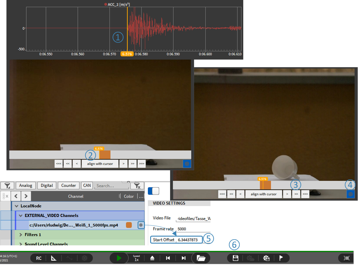
Fig. 342 Alignment of sensor and video data
Use the Recorder to move the orange cursor to the reference event for data synchronization (see ① in Fig. 342)
Press align with cursor to move the video start to the orange cursor position for a rough time adjustment (see ② in Fig. 342)
For fine time adjustments, use the <<<, <<, < & >, >>, >>> buttons to align the timeline (see ③ in Fig. 342)
When finished, the timebar can be hidden (see ④ in Fig. 342)
The absolute time offset can also be seen in the video‘s channel setup (see ⑤ in Fig. 342)
The settings can be saved to the data file (see ⑥ in Fig. 342)
Note
Only the file path to the video is stored to the OXYGEN data file but not the video itself.
Replaying the data file
Details can be found in Reviewing a Data File (PLAY mode).
Saving the measurement screen to video
Details can be found in Saving the screen as video.
DXD import
In OXYGEN Viewer (PLAY mode) it is possible to import *.dxd or *.d7d (②) data as a channel. Data can be shifted by relative time, moved to 1st sample of dmd or aligned on absolute time (③). Both synchronous and asynchronous time domain channels are supported.
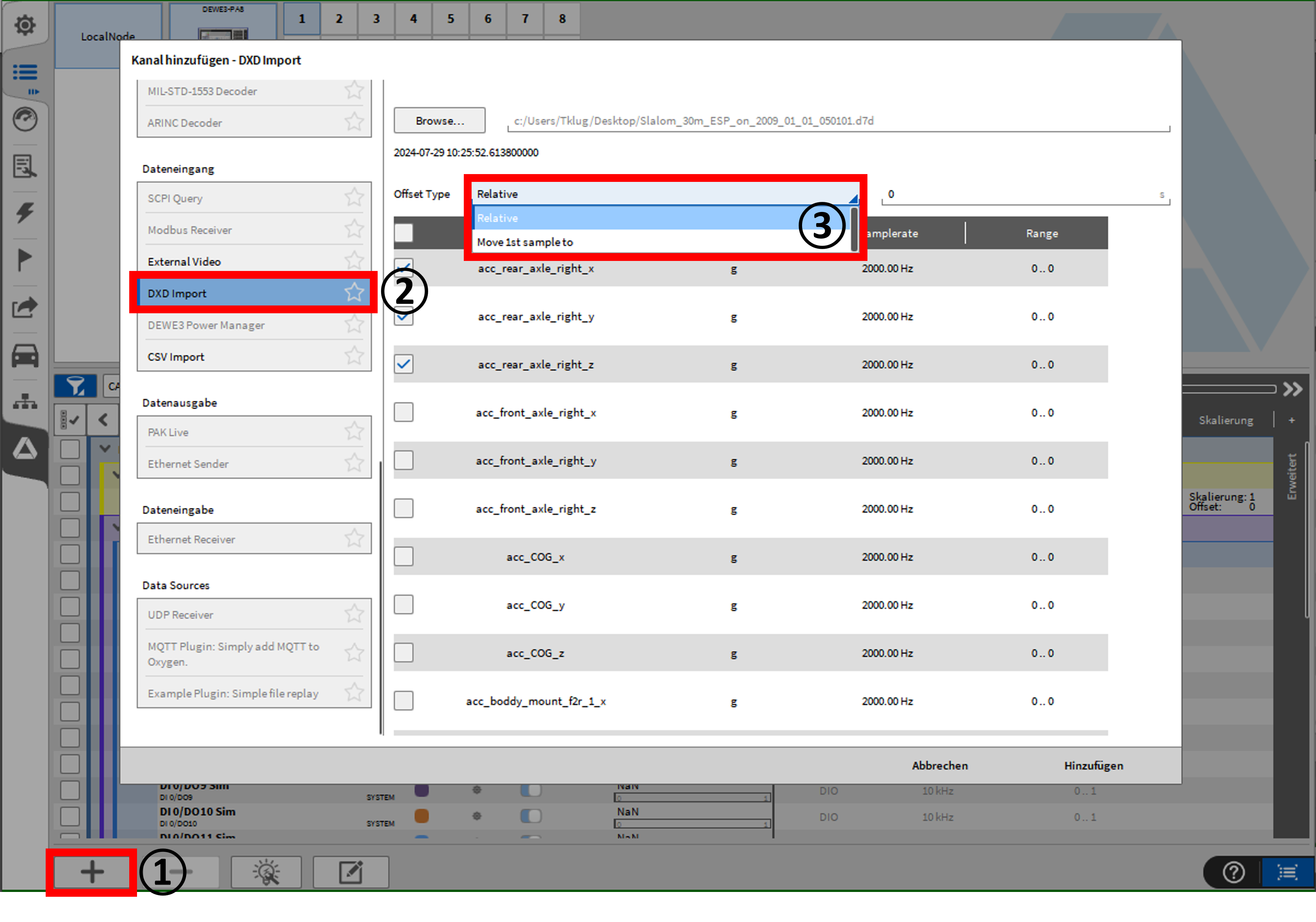
Fig. 343 DXD import
In OXYGEN Viewer (PLAY mode) it is possible to import *.dxd or *.d7d (②) data as a channel. Data can be sifted by relative time and absolute time (③). Both synchronous and asynchonous time domain channels are supported.
CSV/TXT import
In OXYGEN Viewer it is possible to import CSV or TXT data as a channel. This is only available in PLAY mode (see ① in Fig. 344). The first column can be interpreted as relative or absolute time (see ③ in Fig. 344). The Equidistant option allows asynchronous data to be read in with a virtual sampling rate. In case no time is included a synchronous sample rate can be defined (see ④ in Fig. 344). An optional time offset can be defined before adding the channel (see ⑤ in Fig. 344) or subsequently in the properties (see ⑥ in Fig. 344). The imported channel can be found in the group CSV_TXT_IMPORT Channels in the channel list.
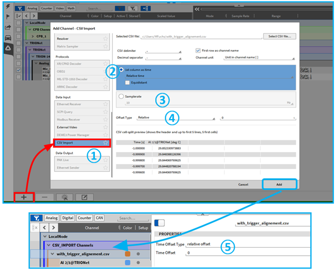
Fig. 344 CSV/TXT import
Data output
PAK Live
This option allows data to be sent from OXYGEN to the PAK live.hub of MBBM.
For details about the PAK Live plugin refer to the OXYGEN PAK Live manual which is available on the DEWETRON CCC portal.
Ethernet Sender
This option allows data from OXYGEN to be output via UDP.
Details about the Ethernet Sender plugin can be found in the OXYGEN Ethernet sender manual, which is available on the DEWETRON CCC portal.
Offline math
The topology Offline Math deems calculations that shall be performed after the measurement is finished within a data file (.dmd). The following Offline Math features are supported. The features will be extended within the proximate OXYGEN releases.

Fig. 345 Editing of already stored channels
The “Edit already stored channels” button (see Fig. 345) software channels, such as formulas, statistics or power groups, which were calculated during recording, can also be modified offline. Dependencies of these channels are updated automatically. Additionally, it is also possible to change the name as well as the unit of hardware channels offline.
Offline Math is not applicable for the scaling of an analog input channel.
Channels can be added afterwards in the same manner as explained in Software channels by clicking on the + button (see Fig. 224) at the lower left side of the Channel List.
Channels created or edited within one open session can be deleted by clicking on the Delete Math Channel button (see Table 10). After re-opening a data file, the previously created channels cannot be deleted any more.
Formulas, Filters, Statistics, FFT channels, the Psophometer plugin, the Swept Sine Analysis plugin, the Rosette determination, the sound level option and the CPB analysis can be used offline as well.
Channel dependencies are respected during Offline Math calculations. This denotes that it is possible to create a Filter channel and a Statistics Channel that is applied on this certain Filter channel within one session. If the Filter channel is edited again, the Statistics channel will automatically be recalculated, too.
Channels that have been created offline can be recognized on the Green Record button in the Channel List (see Fig. 346):
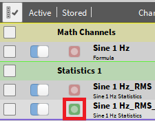
Fig. 346 Recognition of offline created channels
Created channels and any changes can be stored to the data file by pressing the Store data button (see Fig. 347 or ⑬ in Fig. 14):

Fig. 347 Store data button
Created channels and any changes can be exported to a setup file by pressing the Save setup file button (see Fig. 348 or ⑮ in Fig. 14):

Fig. 348 Save setup file button
A Progress indicator will inform about the actual calculation progress (see Fig. 349) and contains information about the number of calculated channels, the calculation progress in percent and the remaining calculation time:
Fig. 349 Progress indicator for Offline Math calculations
A data file recorded with OXYGEN 2.x can be opened with OXYGEN 3.x to apply Offline Math. After storing changes to the data file, it cannot be opened with OXYGEN 2.x again but only with OXYGEN 3.x.
Be aware that an Offline Statistics channel will differ from an Online Statistics channel, i.e. at the beginning of the file or in case of Event based waveform recording (see Triggered Events). In the example displayed in Fig. 350, the green channel is an online calculated Statistics channel applied on the yellow analog channel and the red channel is an offline calculated Statistics channel applied on the yellow analog channel with identical channel settings. The deviation of the green and the red channel is due to the availability of the full analog data during online calculation. During the offline calculation, only the event based recorded analog data is available.
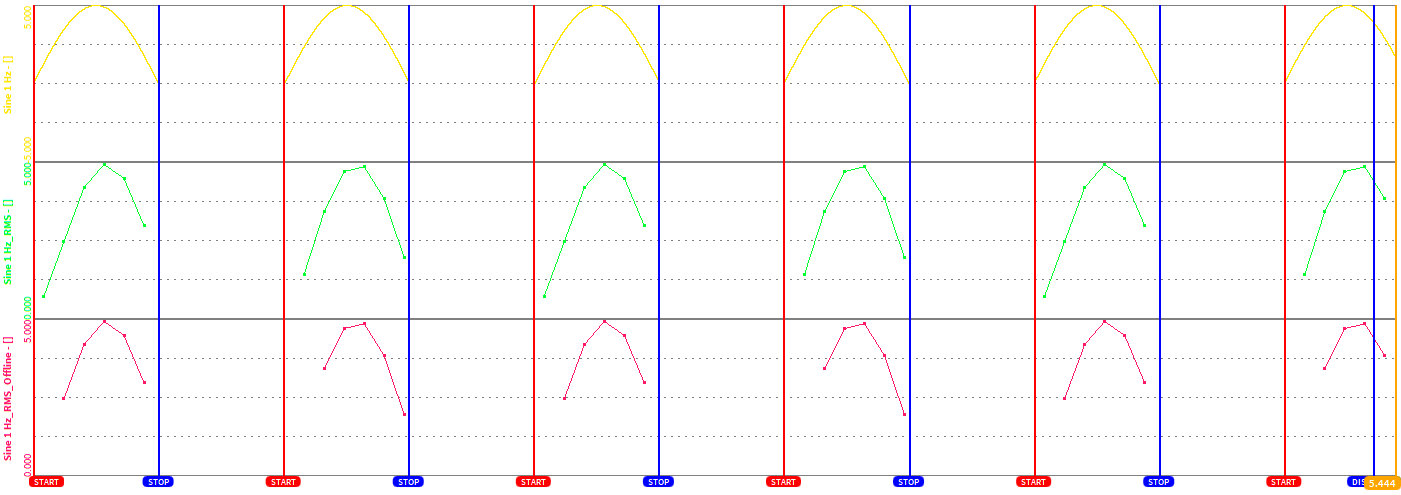
Fig. 350 Deviation of Offline and Online Statistics channels in case of Event based Waveform recording
Be aware that an Offline Filter channel will differ from an Online Filter channel, i.e. at the beginning of the file or in case of Event based waveform recording (see Triggered Events). In the example displayed in Fig. 351, the green channel is an online calculated Integrator applied on the yellow analog channel and the red channel is an offline calculated integrator applied on the yellow analog channel with identical channel settings. The deviation of the green and the red channel happens, because the offline calculated integrator will oscillate at the beginning of each new event, but the online calculated integrator not, because the analog data is always available during online calculation.
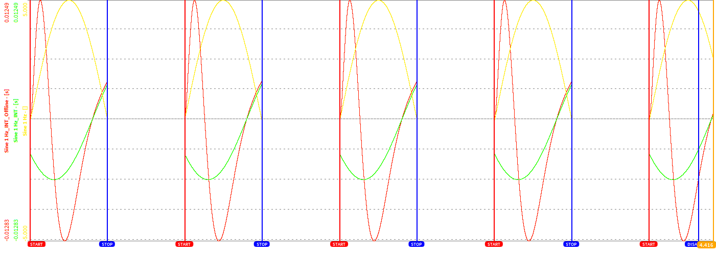
Fig. 351 Deviation of Offline and Online Filter channels in case of Event based Waveform recording
Digital Input/Output modes of the chassis controller
The mode of digital input channels is fixed to Digital In. Starting with TRION / OXYGEN 8.1, the digital output channels of the chassis controller can be configured to different output modes. The following Output Modes are available:
Digital Out - Outputs a static digital signal
Low or High
FrequencyClock - Outputs a configurable clock signal.
Frequency: 1 Hz … 10 MHz
Continous Output (True/False): True → signal is output continuously without resetting at measurement start
Invert signal (True/False): True → signal starts High instead of Low
IRIG - Outputs an IRIG time signal.
Source: IRIG_GEN (static setting)
Code: CodeB_DC (static setting)
Note
The IRIG digital output mode is only available if IRIG is selected either in the Sync Settings or for the Digital AUX channel.
PPS - Outputs a Pulse-Per-Second signal.
CLK10 - Outputs a 10 MHz Clock
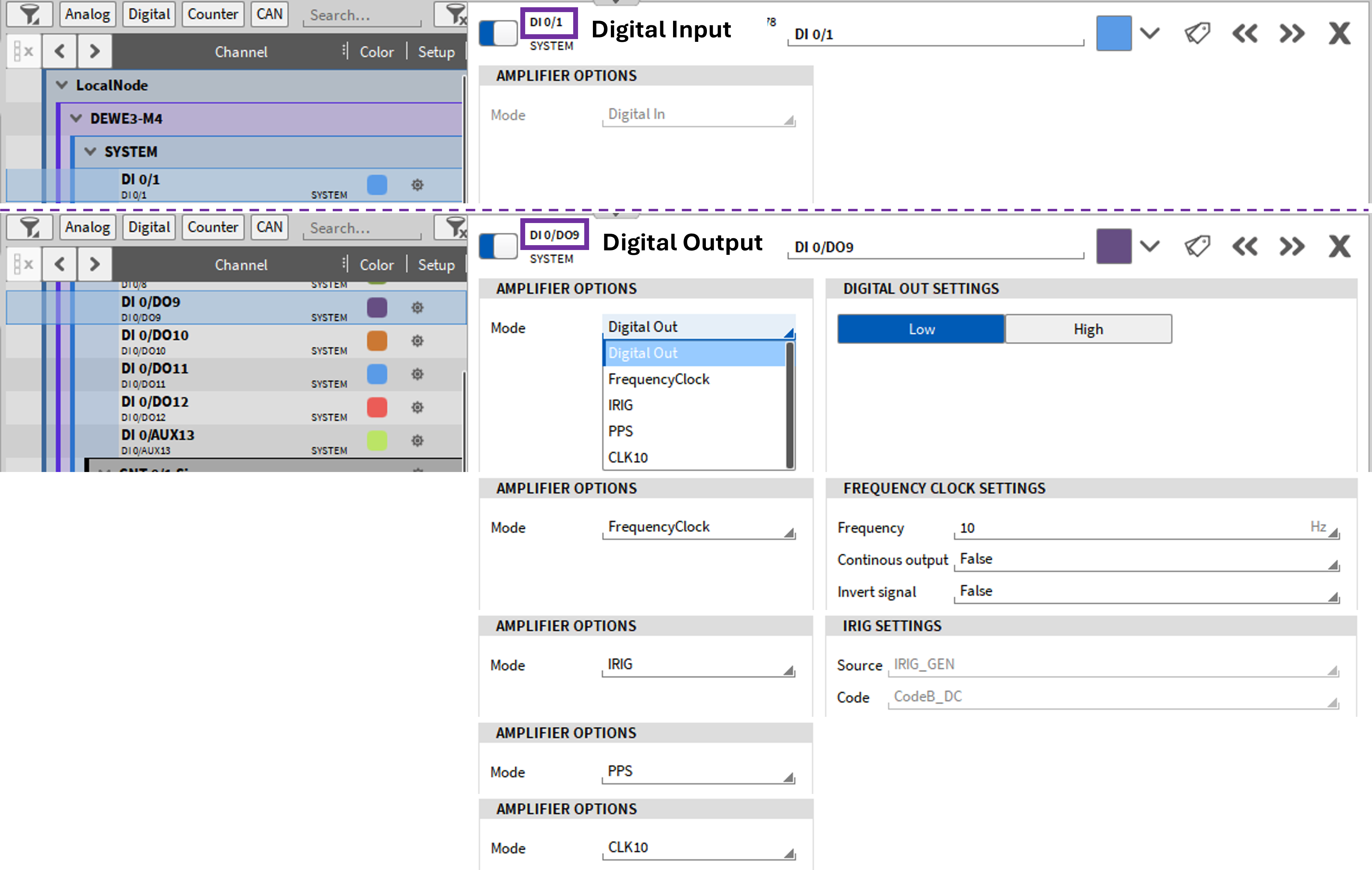
Fig. 352 Digital Output modes for the chassis controller.
Note
For these digital out features the firmware of >R8.1 TRION Applications is required.
AUX output modes of the Chassis Controller
Starting with TRION / OXYGEN 8.1, the AUX output connector is available in the channel list. The following output modes are available:
Setting the output mode of the AUX output in the channel list, restricts the settings in the synchronization setup. The default AUX setting CustomSignalOut means, the setting of the synchronization setup is applied.
CustomSignalOut
Disabled - Output of AUX bin is defined by synchronization setup
PPS - Outputs a Pulse-Per-Second signal.
FrequencyClock - Outputs a configurable clock signal.
Frequency: 1 Hz … 10 MHz
Continous Output (True/False): True → signal is output continuously without resetting at measurement start
IRIG - Outputs an IRIG time signal.
Source: IRIG_GEN (static setting)
Code: CodeB_DC (static setting)
Note
The IRIG digital output mode is only available if IRIG is selected either in the Sync Settings or for the Digital AUX channel.
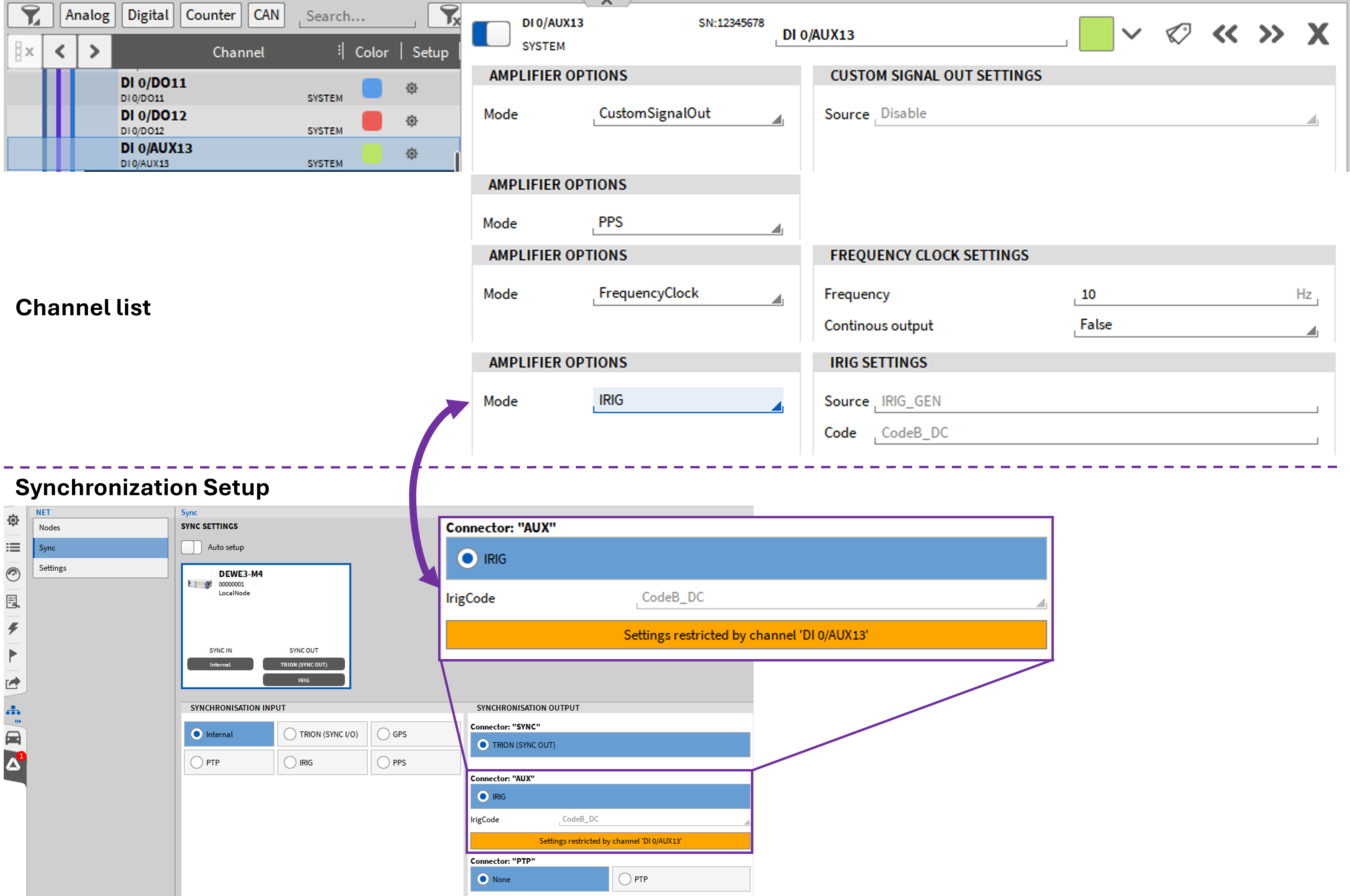
Fig. 353 AUX Output modes for the chassis controller.
Note
Selecting any AUX output mode (besides CustomSignalOut) in the channel list overrides the corresponding settings in the Synchronization Setup. For these AUX features the firmware of >R8.1 TRION Applications is required.
Counter Channels in OXYGEN
OXYGEN supports three different Counter modes: Event Counting, Frequency determination and Encoder Mode (incl. X1, X2, X4 and A-up / B-down) counting.
The following extract from TRION module Technical Reference Manual provides an explanation of the different counting modes. For detailed information, refer to the TRION module Technical Reference Manual.
Counter Modes
Event counting
In Event Counting, the counter counts the number of pulses that occur on input A/B. At every acquisition clock, the counter value is read without disturbing the counting process.
Fig. 354 shows an example of event counting where the counter counts eight events on Input A or B. Synchronized Value is the value read by the TRION-CNT module at Acquisition Clock (encircled numbers in the figure, e.g. 1, 2).
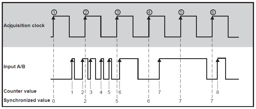
Fig. 354 Event Counting
If counting at falling edges is necessary, the input signal must be inverted. This can be done directly in the software by selecting inverted input.
Frequency measurement
In general, it is possible to take the inverse of a period measurement to get the frequency of the input signal. If the period time measurement is done, an inaccuracy of counted internal time base cycles of ±1 cycle appears, because the counted cycles of the internal time base depend on the phase of the input signal with respect to the internal time base. For long period times, and therewith low frequencies, the measurement error is negligible. At high frequencies, and therewith short period times, few cycles are counted. In this case the error of ±1 cycle becomes significant.
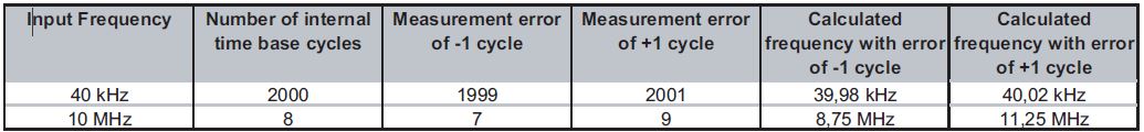
Fig. 355 Accuracy at period time measurement
For higher precision result, a combination of main and sub counter is used internally for getting higher precision at the frequency measurement. The main counter is running on event counting (or encoder mode). The sub counter measures the time between. The sub counter measures exactly the time of the input event with a resolution of 12.5 ns relative to the acquisition clock. At every rising edge on Input A the counter value of the sub counter is stored in a register. At every Acquisition Clock (1, 2, …,6) the values of both counters are read out.
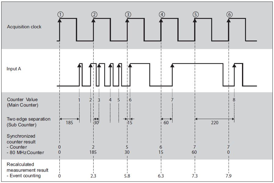
Fig. 356 Frequency measurement
Pulse width measurement
In Pulse Width Measurement the counter uses the internal time base to measure the pulse width of the signal present on Input A. The counter counts the rising edges of the internal time base after a rising edge occurs on Input A. At the falling edge on Input A the counter value is stored in a register and the counter is set to zero. With the next rising edge on Input A the counter starts counting again. At every Acquisition Clock ( 1 , 2 , …, 6 ) the register value is read out.
Fig. 357 shows a pulse width measurement.
Note
For measuring the low time of the signal, the input signal has to be inverted on the TRION-CNT module.
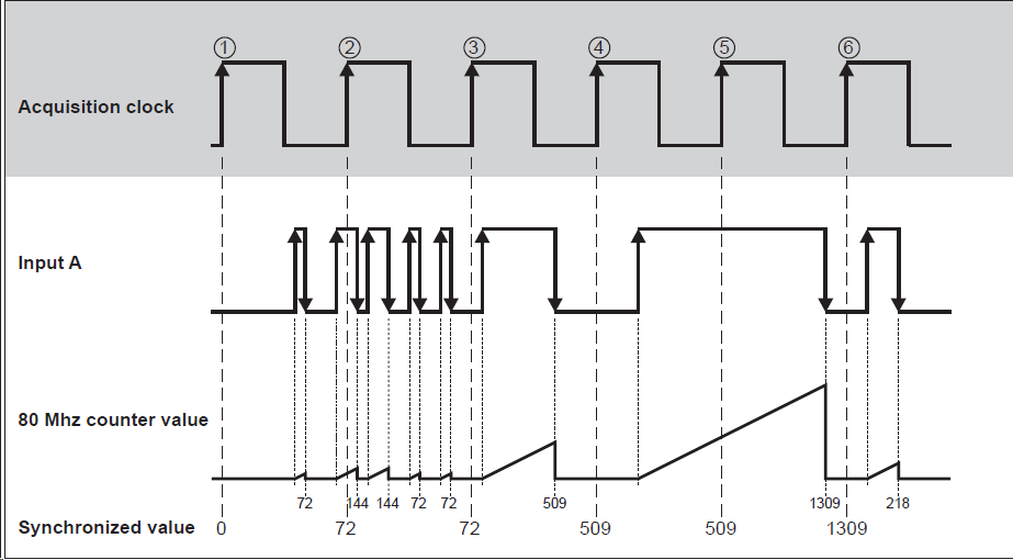
Fig. 357 Pulse width measurement
Encoder
Motion encoders have usually three channels: channel A, B and Z. Channel A and channel B are providing the square signals for the counter and have a phase shift of 90°. With this phase shift, the decoder can recognize the rotation direction of the motion encoder. The third channel types out one pulse at a certain position at each revolution. This pulse is used to set the counter to zero. The amount of counts per cycle at a given motion encoder depends on the type of decoding: X1, X2, X4. All three types are provided by the TRION-CNT module. Some motion encoders have two outputs, which are working in a different way. Either channel A or channel B providing the square signal, depending on the direction of the rotation. Also, this type is supplied by the TRION-CNT module.
In the first case X1 decoding is explained. When Input A leads Input B in a quadrature cycle, the counter increments on rising edges of Input A. When Input B leads Input A in a quadrature cycle, the counter decrements on the falling edges of Input A. At every Acquisition Clock (1, 2, …, 9), the counter value is read out.
Fig. 358 shows the resulting increments and decrements for X1 encoding.
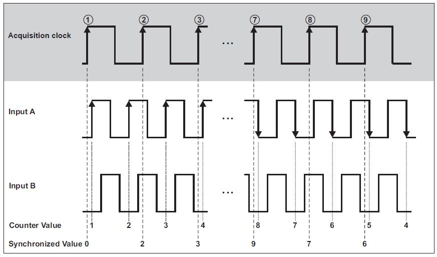
Fig. 358 Quadrature Encoder X1 Mode
For X2 encoding, the rising edges and the falling edges of Input A are used to increment or decrement. The counter increments if Input A leads Input B and decrements if Input B leads Input A. This is shown in Fig. 359.
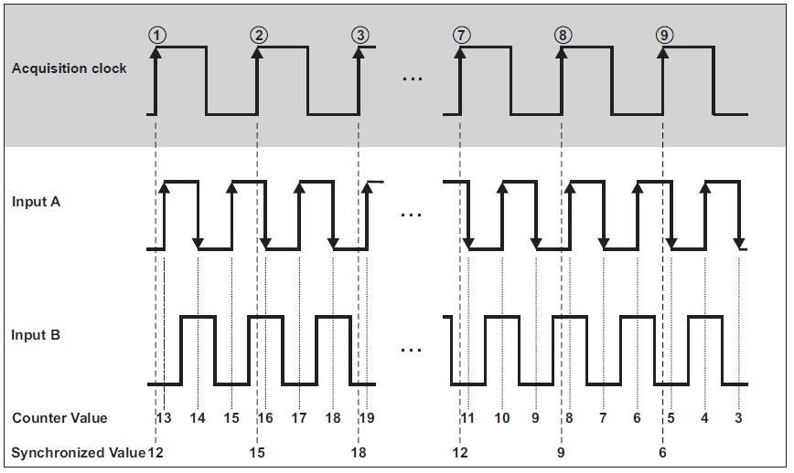
Fig. 359 Quadrature Encoder X2 Mode
Similarly, the counter increments or decrements on each edge of Input A and Input B for X4 decoding. The condition for increment and decrement is the same as for X1 and X2.
Fig. 360 shows the results for X4 encoding.
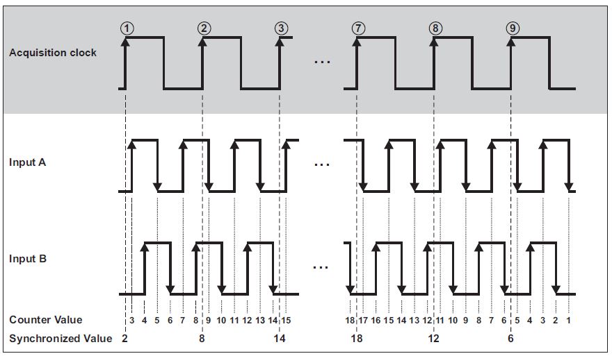
Fig. 360 Quadrature Encoder X4 Mode
The third channel Input Z, which is also referred as the index channel, causes the counter to be reloaded with zero in a specific phase of the quadrature cycle.
Fig. 361 shows the results for X1 encoding with input Z.
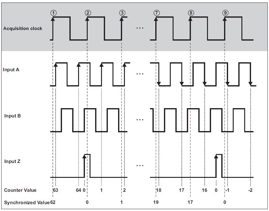
Fig. 361 Quadrature Encoder with channel Z
The A-Up/B-Down Encoder supports two inputs, A and B. A pulse on Input A increments the counter on its rising edges. A pulse on Input B decrements the counter on its rising edges. At every Acquisition Clock (1, 2, …, 9), the counter value is read out.
This situation is shown in Fig. 362.
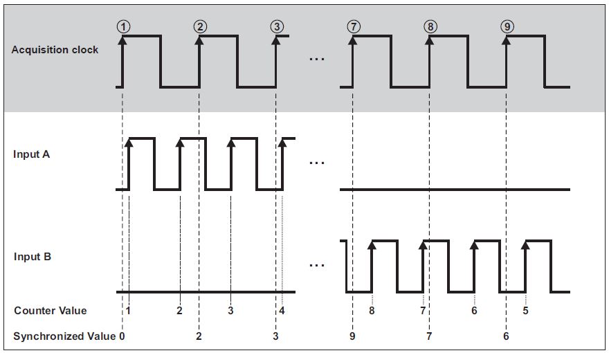
Fig. 362 A-Up/B-Down Encoder
TRION Counter Overview
TRION |
-CNT |
-BASE |
-TIMING |
-VGPS |
-1620-ACC |
-2402-dACC |
(3)-18x0-MULTI |
-1802/1600-dLV |
|---|---|---|---|---|---|---|---|---|
#Counter #Inputs/counter |
6 3 |
2 3 |
1 3 |
1 3 |
1 1 |
2 1 |
2 1 |
1 3 |
Isolation |
✓ |
x |
x |
x |
✓ |
x |
✓ |
x |
Trigger level |
0 to 50 V / 12 mV steps |
CMOS/TTL |
CMOS/TTL |
CMOS/TTL |
70 % of input range |
Progr. within input range |
75 % of input range |
CMOS/TTL |
Event counting |
✓ |
✓ |
✓ |
✓ |
✓ |
✓ |
✓ |
✓ |
Frequency/pulse width measurement |
✓ |
✓ |
✓ |
✓ |
✓ |
✓ |
✓ |
✓ |
Encoder support |
✓ |
✓ |
✓ |
✓ |
x |
x |
x |
✓ |
Angle determination (SW) |
✓ |
✓ |
✓ |
✓ |
✓ |
✓ |
✓ |
✓ |
Speed determination (SW) |
✓ |
✓ |
✓ |
✓ |
✓ |
✓ |
✓ |
✓ |
Sensor supply |
5 and 12 V |
5 and 12 V |
5 and 12 V |
5 and 12 V |
x |
x |
x |
5 and 12 V |
As shown in Table 41, Frequency measurement and Event counting can be done with every TRION module with counter input. Encoders and CDM+Trigger sensors cannot be connected to a the TRION-1620-ACC or the TRION-2402-dACC module as they don’t have several digital input channels per counter channel. Hence, angle and rpm measurements are possible with a counter channel of a TRION-1620-ACC or TRION-2402-dACC module, but no turning direction can be determined.
Note
The Trigger Level supported by the TRION-2402-dACC module differs from the software possibilities.
Channel List of Counter Channels
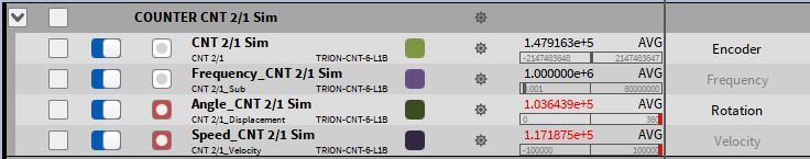
Fig. 363 Channel List of a Counter channel
4 single sub-channels are created for each available Counter channel (COUNTER CNT 2/1 Sim in Fig. 363)in the Channel List. The counter hardware of one Counter channel (except TRION-dACC and TRION-ACC hardware) consists of two different counter logics, the Main counter and the Sub counter (see Fig. 364).
The first sub-channel (CNT 2/1 Sim in Fig. 363) is linked to the Main counter. If the Counter channel shall be used in the Event Counting or Encoder mode (X1, X2, X4, A-up/B-down), it must be defined in the Channel Setup of this sub-channel. The Frequency mode can be selected in this sub-channel as well, but this is only due to guarantee the compatibility with old setup files. The sub-channels 3 and 4 will disappear if the Frequency mode is selected (Angle_CNT2/1 Sim and Speed_CNT 2/1 Sim in Fig. 363).
The second sub-channel (Frequency_CNT 2/1 Sim in Fig. 363:) is linked to the Sub counter. This channel is used for the frequency measurement. If Frequency mode is selected in sub-channel one (CNT 2/1 Sim in Fig. 363), sub-channel two (Frequency_CNT 2/1 Sim in Fig. 363) is deactivated and does not display data.
The third sub-channel (Angle_CNT 2/1 Sim in Fig. 363) calculates the angle by using the data acquired from the Main counter and Sub counter logic and the fourth sub-channel (Speed_CNT 2/1 Sim in Fig. 363) calculates the speed by using the data acquired from the Main counter and Sub counter logic.
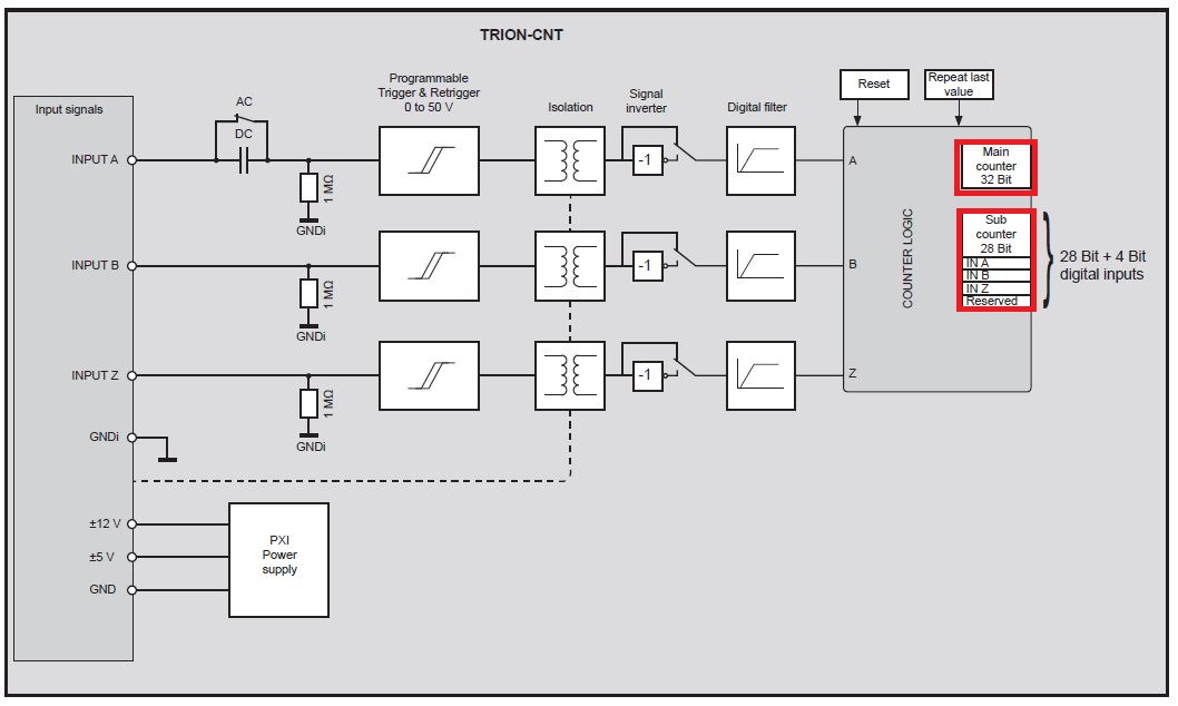
Fig. 364 Block diagram of one Counter channel on a TRION-CNT module
Note
The maximum bus data rate of 90 MB/s is reached if 6 channels of a TRION-CNT module are stored with 2 MHz Sample Rate.
Channel Setup of a Counter Channel
Each of the four sub-channels has an own Channel Setup. The Channel Setups of all 4 sub-channels is summarized in the Channel Setup of the main counter channel (COUNTER CNT 2/1 Sim in Fig. 365) and can be entered by clicking on the gear button (see Fig. 365). The scaling of a sub-channel can be changed in the Channel Setup of the individual sub-channel.
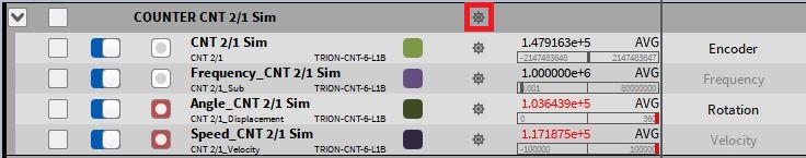
Fig. 365 Channel setup of a Counter channel
In the following, the Channel Setup of a Main Counter channel for and its options for an Event mode and an Encoder mode are explained on the example of a TRION-CNT module. Due to limited hardware possibilities, the channel setup of a TRION-ACC or TRION-dACC module counter channel provides less options.
Channel Setup for a TRION-CNT Channel in Event mode
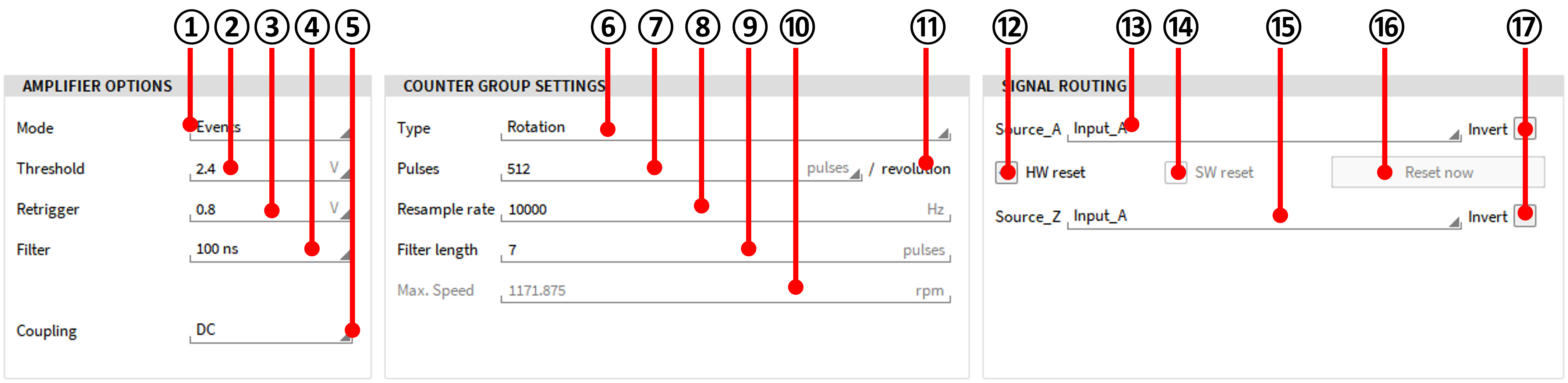
Fig. 366 Channel Setup for a TRION-CNT channel in Event mode
No. |
Function |
Description |
|---|---|---|
Amplifier Options |
||
1 |
Mode menu |
Counter mode selection: Events, Frequency or Encoder |
2 |
Threshold level |
Threshold (Trigger) Level selection (depends on the TRION hardware, see Table 41) |
3 |
Retrigger level |
Retrigger Level selection (depends on the TRION hardware, see Table 41) |
4 |
Filter menu |
Selection of a digital filter; for additional information refer to Digital Filter of a Counter Channel |
5 |
Coupling menu |
Coupling (HP filter) selection (availability depends on TRION hardware) |
Counter Group Settings |
||
6 |
Type menu |
Decoding type: Rotation or Linear decoding type |
7 |
Pulses selection |
Number of pulses transmitted by the counter per revolution, meter, … |
8 |
Resample rate selection |
Select the Resample rate here; needed if time synchronous counter and analog data is required. Enter the sample rate of the analog channel here and counter data will be time synchronous to the analog data |
9 |
Filter length |
Apply a moving average filter on speed by number of pulses. For speed signal smoothing without delay. Applicable in Event and Encoder mode. |
10 |
Maximum speed |
Maximum recommended speed calculated by sample rate (per minute) divided by pulses per revolution. Max. speed [rpm] = Sample rate [Hz] x 60 / pulses per revolution |
11 |
Unit selection |
Unit selection; for rotational sensors fixed to revolution, set to meters per default for linear sensors |
Signal Routing |
||
12 |
HW Reset button |
HW reset selection; If this option is selected, a second input Source_Z must be selected. Source_A channel is reset if the edge of Source_Z raises from 0 to 1 |
13 |
Source_A selection |
Select the input signal that shall be routed to Source_A |
14 |
SW Reset button |
SW Reset selection; If this option is selected, Source_A is reset after the number of pulses entered in ⑦ is reached |
15 |
Source_Z selection |
Select the input signal that shall be routed to Source_Z (only applicable if HW Reset is selected) |
16 |
Reset now button |
If this button is pressed, a manual hardware reset is forced |
17 |
Invert channel button |
Inverts the respective input channel |
Note
An automatic Counter Reset at Recording Start is not supported
Channel Setup for a TRION-CNT Channel in Encoder mode
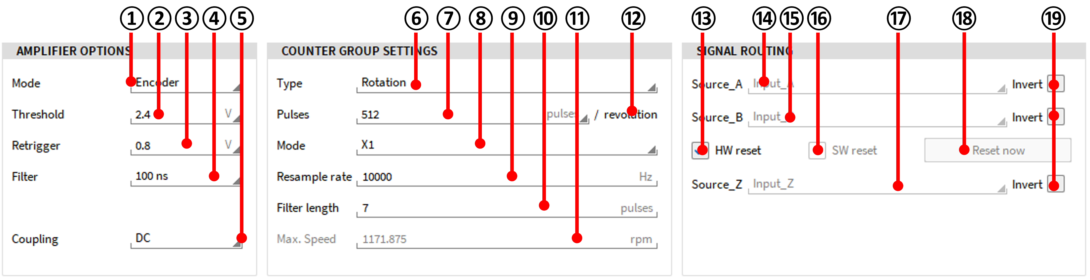
Fig. 367 Channel Setup for a TRION-CNT channel in Encoder mode
No. |
Function |
Description |
|---|---|---|
Amplifier Options |
||
1 |
Mode menu |
Counter mode selection: Events, Frequency or Encoder |
2 |
Threshold level |
Threshold (Trigger) Level selection (depends on the TRION hardware, see Table 41) |
3 |
Retrigger level |
Retrigger Level selection (depends on the TRION hardware, see Table 41) |
4 |
Filter menu |
Selection of a digital filter; for additional information refer to Digital Filter of a Counter Channel |
5 |
Coupling menu |
Coupling (HP filter) selection (availability depends on TRION hardware) |
Counter Group Settings |
||
6 |
Type menu |
Decoding type: Rotation or Linear decoding type |
7 |
Pulses selection |
Number of pulses transmitted by the counter per revolution, meter, … |
8 |
Encoder Mode selection |
Select the Encoder mode: X1, X2, X4, A-Up/B-Down |
9 |
Resample rate selection |
Select the Resample rate here; needed if time synchronous counter and analog data is required. Enter the sample rate of the analog channel here and counter data will be time synchronous to the analog data |
10 |
Filter length |
Apply a moving average filter on speed by number of pulses. For speed signal smoothing without delay. Applicable in Event and Encoder mode. |
11 |
Maximum speed |
Maximum recommended speed calculated by sample rate (per minute) divided by pulses per revolution. Max. speed [rpm] = Sample rate [Hz] x 60 / pulses per revolution |
12 |
Unit selection |
Unit selection; for rotational sensors fixed to revolution, set to meters per default for linear sensors |
Signal Routing |
||
13 |
HW Reset button |
HW reset selection; If this option is selected, a second input Source_Z must be selected. Source_A channel is reset if the edge of Source_Z raises from 0 to 1 |
14 |
Source_A selection |
Displays the signal that is routed to Source_A (routing can’t be edited in the Encoder mode) |
15 |
Source_B selection |
Displays the signal that is routed to Source_B (routing can’t be edited in the Encoder mode) |
16 |
SW Reset button |
SW Reset selection; If this option is selected, Source_A is reset after the number of pulses entered in ⑦ is reached |
17 |
Source_Z selection |
Displays the signal that is routed to Source_Z (only applicable if HW Reset is selected, routing can’t be edited in the Encoder mode) |
18 |
Reset now button |
If this button is pressed a manual hardware reset is forced |
19 |
Invert channel button |
Inverts the respective input channel |
Note
An automatic Counter Reset at Recording Start is not supported
Digital Filter of a Counter Channel
Each counter and digital input has a digital filter, which can be set to various gate times. If the gate time is set to “Off”, no filter is on the input signal. The filter circuit samples the input signal on each rising edge of the internal time base. If the input signal maintains his state for at least the gate time, the new state is propagated. As an effect the signal transition is shifted by the gate time.
Fig. 368 demonstrates the function of the filter.
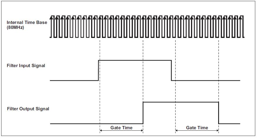
Fig. 368 Digital filter
The intent of the filter is to eliminate unstable states, e.g. glitches, jitter… which may appear on the input signal, as shown in Fig. 369.
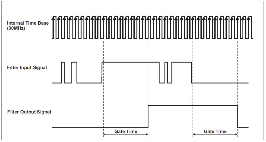
Fig. 369 Input signal with chatter
It can be chosen between eight filter settings: Off, 100 ns, 200 ns, 500 ns, 1 μs, 2 μs, 4 μs and 5 μs. Two examples of filter settings are described. The 100 ns filter will pass all pulse widths (high and low) that are 100 ns or longer. It will block all pulse widths that are 75 ns or shorter. The 5 μs filter will pass all pulse widths (high and low) that are 5 μs or longer and will block all pulse widths that are 4.975 μs or shorter. The internal sampling clock (time base) is 80 MHz, so the period time amounts 12.5 ns. Pulse widths between gate time minus two internal time base period times may or may not pass, depending on the phase of the input signal with respect to the internal time base.
Properties of all filter settings:
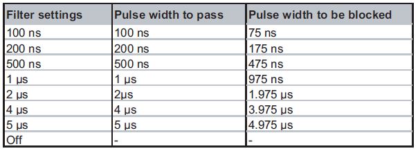
Fig. 370 Filter Gate Times
Supported Counter Sensors
Due to the software and TRION-hardware possibilities, OXYGEN supports three different types of counter sensors: Tacho sensors, CDM+Trigger sensors and Encoder sensors. The following table provides an overview about the possibilities and differences of the different types of sensors:
Mounting |
Connect |
Pulses |
Frequency |
Required digital counter inputs |
Measurement |
|||
|---|---|---|---|---|---|---|---|---|
RPM |
Angle |
Direction |
||||||
Tacho |
Easy |
Analog or adj. CNT |
1 kHz |
0.1 |
1 |
✓ |
x |
x |
CDM+ Trigger |
Hard |
CNT |
360/720/xxx |
125 kHz |
2 |
✓ |
✓ |
x |
Encoder coder |
Hard |
CNT |
Up to 36000 and more |
~100 kHz |
3 |
✓ |
✓ |
✓ |
Mandatory channel settings for Tacho sensors
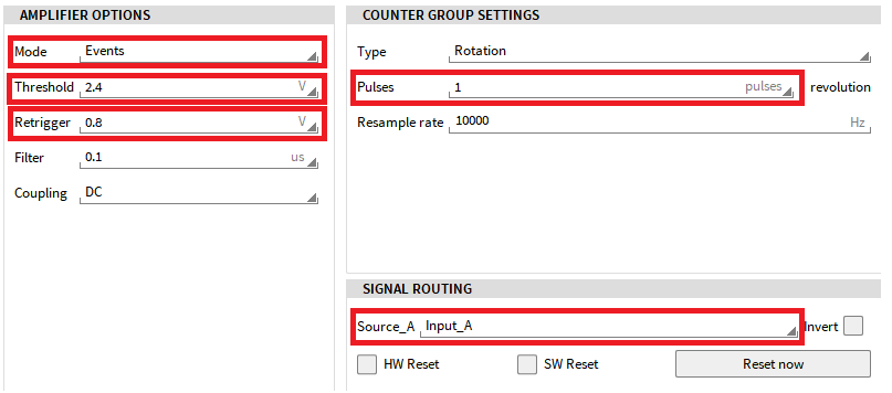
Fig. 371 Channel settings for a Tacho sensor
Amplifier Mode must be set to Events
Threshold and Retrigger Level must be adjusted depending on the sensor signal
Number of Pulses must be set to 1 pulse /revolution
Sensor signal must be routed to Source_A
Mandatory channel settings for CDM+Trigger sensors
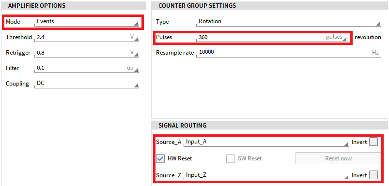
Fig. 372 Channel settings for a CDM +Trigger sensor
Amplifier Mode must be set to Events
Number of Pulses per revolution provided by the CDM signal must be entered
Route the CDM signal to Source_A and the Trigger signal to Source_Z (HW reset must be enabled)
Note
The Amplifier Mode can also be set to Encoder. In this case, the same settings as in Fig. 373 are mandatory. Note that the routing of the Source_A and Source_B input cannot be changed.
Mandatory channel settings for Encoder sensors
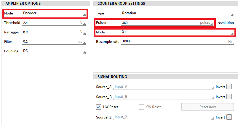
Fig. 373 Channel settings for an Encoder sensor
Amplifier Mode must be set to Encoder
Number of Pulses per revolution provided by the Input_A and Input_B must be entered
The counting mode X1, X2, X4 or A-Up/B-Down must be selected
CAN Input Channels
The following TRION-boards provide one or several CAN ports
TRION-CAN: 2 or 4 ports
TRION(3)-18x0-MULTI: 1 CAN port
TRION-2402-MULTI: 1 CAN port
TRION-1600-1802-dLV-CAN: 1 CAN port
In addition, Vector devices from the VNxxxx series (i.e. VN1610 or VN7610) can be used for the CAN data acquisition as well. These devices are the dedicated hardware to also acquire CAN-FD data streams and can therefore be used for CAN data acquisition.
Note
The usage of Vector VNxxxx devices requires a separate software license.
CAN port configuration
To configure the CAN port properly, go to the Channel List and open the CAN port configuration of the dedicated CAN port by pressing the Gear button (see ① in Fig. 374).
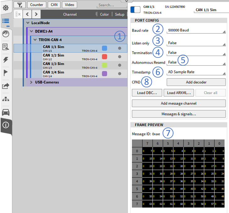
Fig. 374 CAN port configuration
Note
When using the CAN port of a TRION(3)-18x0-MULTI or a TRION-2402—MULTI board, the CAN port is available on AI 1 of these boards. For accessing and using these CAN ports, you have to set the Input mode of AI 1 to CAN first and activate the dedicated CAN port second (see Fig. 375)
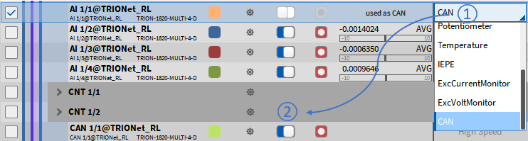
Fig. 375 Using the CAN port of a TRION-MULTI board
The following settings are available:
Baud rate (see ② in Fig. 374):
Select the proper Baud rate of the CAN bus here
Listen only (see ③ in Fig. 374):
With the listen-only mode activated, normal bus activity can be monitored by the device. However, if an error frame is generated by the local CAN controller, it is not transmitted to the bus. Since in listen-only mode the module has no transmit function this feature must not be used in a point-to-point connection.
For more information, refer to the to the TRION series technical reference manual which is available on the DEWETRON CCC-portal (https://ccc.dewetron.com/).
Termination (see ④ in Fig. 374):
TRION-CAN ports offer a programmable termination resistance, either high impedance (False) or 120 Ω (True).
For more information, refer to the to the TRION series technical reference manual which is available on the DEWETRON CCC-portal (https://ccc.dewetron.com/).
Autonomous Resend (see ⑤ in Fig. 374):
Only affects CAN data output. For details, refer to CAN data recording.
Timestamp (see ⑥ in Fig. 374): Sets the time base on which the CAN signals are aligned.
10 MHz:
Assigns a timestamp with 100 ns resolution to the CAN messages and signals. This is the internal time base of the CAN port
AD sample rate:
Assigns the timestamp of the highest analog sample rate to the CAN messages and sig-nals, i.e. 10 kHz analog sample rate results in a timestamp with 100 µs.
100 Hz … 10 MHz:
A user defined CAN timestamp resolution can be defined as well.
The frame preview (see ⑦ in Fig. 374) will show a preview of the received messages if all settings (especially Baud rate and Termination) are set correctly ad data is available on the CAN port.
Additional settings:
CPAD (see ⑧ in Fig. 374): If a module of the CPAD series is connected to the CAN bus, a CPAD decoder can be added for decoding their messages and signals without the need for a proper dbc-file. For more information, refer to Using XRs / CPADs with OXYGEN.
CAN data recording
After configuring the CAN port properly, the CAN stream must be decoded.
Decoding CAN data by using .dbc or .arxml files
The conventional way to decode the CAN data stream is to load either a dbc-file or an arxml-file which includes the information which CAN messages are included in the CAN data stream and how to decode them into CAN signals.
Thus, press Load DBC… (see ① in Fig. 376) or Load ARXML… (see ② in Fig. 376).
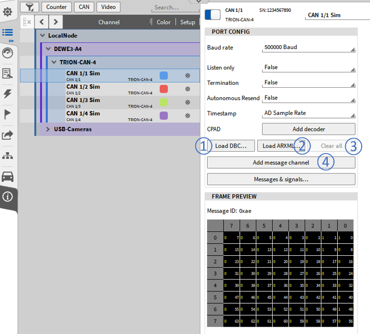
Fig. 376 Decoding CAN data
A file dialog will open to browse and select the proper file.
Note
ARXML file decoding is supported in OXYGEN R5.6 or higher
ARXML file version 4.1 or high is required
After loading the dbc/arxml-file, a channel picker dialog will appear. It is possible to select only dedicat-ed CAN messages and signals for decoding or all channels contained in the file and press Ok afterwards.
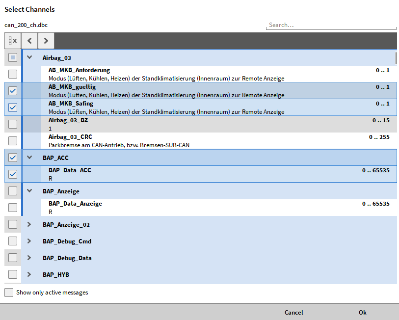
Fig. 377 CAN channel picker dialog
Note
The option Show only active messages performs a scan on the CAN bus to check which CAN messages are available on the CAN bus. You will only see the CAN messages and signals included in the dbc- or arxml-file that are currently available on the CAN bus when this option is activated.
After pressing Ok you will find the selected messages and signals in the channel list (see Fig. 378)
Fig. 378 CAN messages and signals in the Channel List
You can delete all decoded messages and channels by pressing the Clear All button the CAN port config-uration (see ③ in Fig. 376).
If one or several messages available on the CAN bus should not be defined in the selected dbc- or arxml-file you can manually add them by pressing Add message channel (see ④ in Fig. 376) and defining the correct settings in the CAN message setup. More details can be found in CAN message setup.
Note
It is also possible to add and decode other CAN channels from a dbc- or arxml file during the data analy-sis (CAN offline decoding). To do so, the steps above have to be repeated within the loaded data file. The only condition is that the raw CAN data stream was stored during data recording.
CAN message setup
The CAN message setup can be accessed by pressing the gear button of the respective CAN message in the Channel List (see ① in Fig. 379).
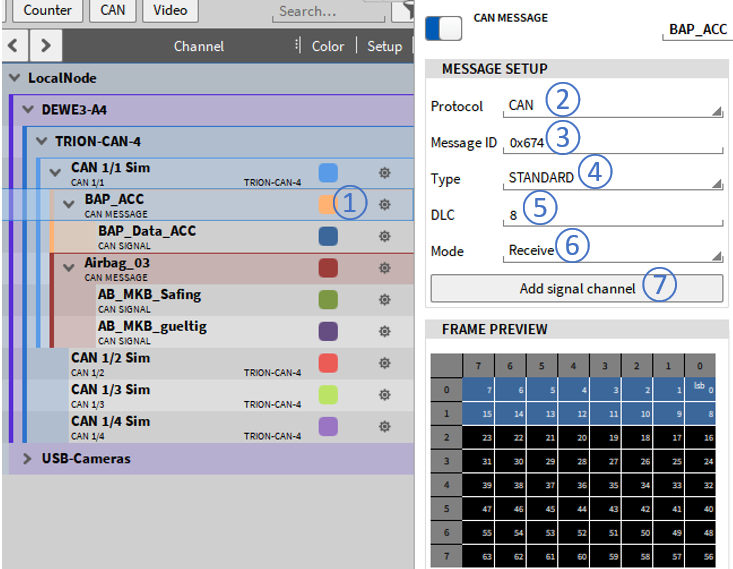
Fig. 379 CAN message channel setup
The following CAN message settings can be edited here if certain settings in the loaded dbc-file were defective:
Protocol type (see ② in Fig. 379): CAN or J1939 or CAN-FD (if applicable)
For additional information about SAE J1939 data decoding, refer to section 4.
Message ID (see ③ in Fig. 379): The message’s ID can be set from 0x00 to 0x7ff
Message Type (see ④ in Fig. 379): Standard or Extended
DLC (see ⑤ in Fig. 379): The DLC can be set from 0 … 8 (…64 for CAN-FD)
Mode (see ⑥ in Fig. 379): The Mode can be set from Receive (Receiving CAN data) to Transmit (Outputting OXYGEN data over CAN).
For additional information, please refer to section 5.
Add signal channel (see ⑦ in Fig. 379):
If the CAN message includes one additional signal which is not loaded from the dbc-or arxml-file or available within the dbc-file, a new signal can be added. The signal’s setting are described in CAN signal setup.
CAN signal setup
The CAN signal setup can be accessed by pressing the gear button of the respective CAN signal in the Channel List (see ① in Fig. 380).
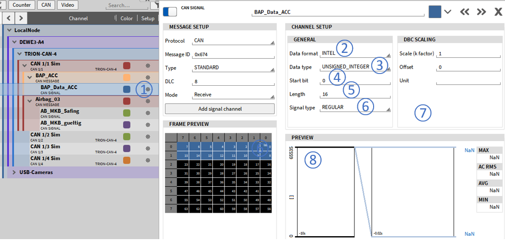
Fig. 380 CAN signal setup
The following CAN signal settings can be edited here if certain settings in the loaded dbc-file were defective:
Data format (see ② in Fig. 380): Intel or Motorola
Data type (see ③ in Fig. 380): Double, Float, Signed Integer or Unsigned Integer
Start bit (see ④ in Fig. 380): Define the start bit of the signal within its message
Length (see ⑤ in Fig. 380): Define the length of the signal within its message
Signal Type (see ⑥ in Fig. 380): Regular, Multiplexed or Multiplexor
DBC Scaling (see ⑦ in Fig. 380): Change the scaling of the signal
Preview: (see ⑧ in Fig. 380): The preview shows the past 10 seconds of the signal to check if proper settings have been applied to the signal.
Signal type
Three different signal types are available in OXYGEN. Signals are the smallest unit of information in a CAN message. The start bit is used to indicate the signal’s position within the message.
Regular: The same signal is transmitted having the same position within the message.
Multiplexed: Different signals are transmitted within the message. The position of the signals is defined using a multiplex value. This value is transmitted in another signal.
Multiplexor: This signal contains the information of the different signal’s positions within the message, which are transmitted as multiplexed signals.
CAN data decoding using the CAN editor
Instead of using .dbc or .arxml files for data decoding it is also possible to add CAN messages and signals manually. OXYGEN provides a CAN editor for this purpose which can be opened by pressing the Messages & signal button the CAN port configuration (see ① in Fig. 381):
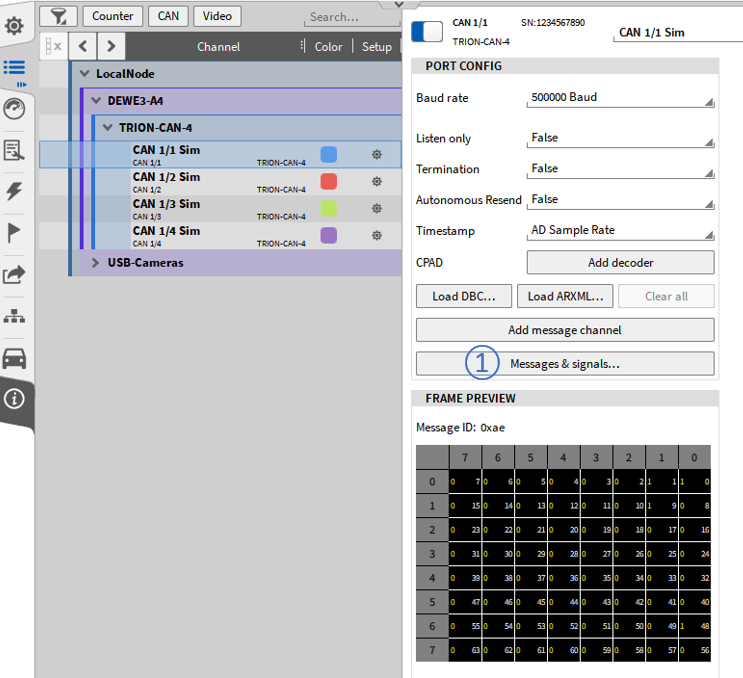
Fig. 381 CAN port configuration
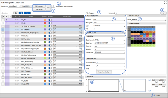
Fig. 382 CAN editor overview
The CAN editor can be used to
Manually add or delete CAN messages and signals (see ① in Fig. 382).
Scan for CAN messages, which will automatically be created with their ID and DLC. After the scan, a name can be given and signals can be created (see ② in Fig. 382).
Rename the currently selected CAN message and signal (see ③ in Fig. 382).
Add comments to messages and signals (see ④ in Fig. 382).
Edit CAN messages and access the same settings as described in section CAN message setup (see ⑤ in Fig. 382). With the enum label editor a text label can be defined for a specific, unique signal value which is then shown in the digital instrument (see also Enum scaling).
Edit CAN signals and access the same settings as described in CAN signal setup (see ⑥ in Fig. 382).
Set the CAN Message mode to Receive for acquiring data or transmit for outputting OXYGEN data over CAN (see ⑦ in Fig. 382).
Providing a preview of the past 10 seconds of the signal to check if proper settings have been applied to the signal (see ⑧ in Fig. 382).
When finished you can exit the CAN editor again by pressing the Close button (see ⑨ in Fig. 382).
Note
The CAN editor and the related CAN message / signal setup is also available for CAN-FD streams.
SAE J1939 DATA DECODING
SAE J1939 is an overlay of standard CAN for primary use in heavy duty vehicles. It uses a standardized messaging system with parameter group numbers encoded in the extended message frame ID.
Main properties
Message ID consists of
PGN-Number
Priority and
Source address
Messages can be longer than standard CAN Frame size due to Multi Frame Messaging system
Decoding of J1939 messages
A simple CAN decoder could receive and decode messages with standard length when the decoder is parametrized with the exact message id. When it comes to practical use, and the user wants to decode and read data with different priority and/or source address, it gets difficult. Also the reading of multi frame messages is not possible with standard tools. OXYGEN supports the Multi Frame Messages as well as decoding messages with varying priority and source address.
Example: DBC-File defines the following Message ID: 0x0CF004FE
PRIORITY (Encoded) = 0x0C >> bit shift 2 = 0x03 (=3)
PGN-Number = 0xF004 (=61444)
Source Address = 0xFE (=254, broadcast)
If a message on the CAN has the following Message ID: 0x18F00400
Standard CAN-Decoder would recognize a different message and does not decode it (because the message ID is not identical to the defined one)
To decode it anyway, OXYGEN ignores the priority and the source address (if it is originally defined as 0xFE)
Frame Description (DBC) |
Decoded in OXYGEN |
|---|---|
PRIO/PGN/SA=0xFE |
0x*PGN** (only PGN matters, source address and priority is ignored) |
PRIO/PGN/SA≠0xFE |
0x*PGN*SA (PGN and Source Address matters, priority is ignored) |
Supported DBC-Formats for Description of J1939 Messages (Requirements):
Correct Specification of the VFrameFormat [J1939 PG (ext. ID)]
BA_DEF\_ BO\_ "VFrameFormat" ENUM "StandardCAN","ExtendedCAN","reserved","J1939PG";
BA_DEF_DEF\_ "VFrameFormat" "J1939PG";
BA\_ "ProtocolType" "J1939";
Each Message must have the VFrameFormat Property 3 (according to ENUM)
BA\_ "VFrameFormat" BO\_ 2633805054 3;
The “Old” format (J1939 PG) is not supported, ask our support, how to convert it to the newer format (J1939 PG (ext. ID)).
Replace Source Address:
If a dbc- or arxml file is loaded that contains J1939 messages, the source Address will be displayed when Show only active messages is activated (see ① in Fig. 383). By Selecting Replace Address it is possible to replace the current source address of the dedicated mes-sage by a user defined one (see ② in Fig. 383).
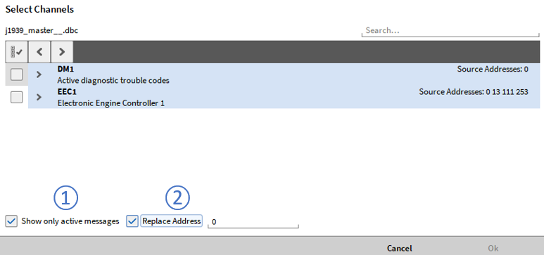
Fig. 383 Channel picker for SAE J1939 messages and signals
CAN-OUT - transmitting OXYGEN data via CAN
Note
This is an optional feature and requires a license.
It is possible to transmit OXYGEN channels cyclically over the CAN bus. This functionality is supported by all CAN ports available on the different TRION boards and also by the Vector VN series CAN ports. For transmitting CAN data, it is either possible to load a dedicated dbc file or to define the CAN messages and signals individually by using the CAN editor. To transmit OXYGEN data over CAN, the CAN message Mode must be set to Transmit (see ① in Fig. 384) for that.
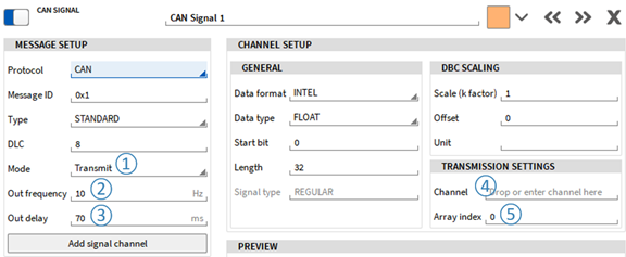
Fig. 384 CAN output settings
The output rate can be defined from 0.1 … 100 Hz (see ② in Fig. 384) individually for each message. The output delay can be set from 1 … 500 ms (see ③ in Fig. 384). One dedicated OXYGEN scalar time domain channel (i.e. Analog or Digital input, power value such as Active power or another CAN channel) can be assigned to one CAN signal by dropping the channel or typing its name into the Channel section of Transmission settings (see ④ in Fig. 384).
It is also possible to output dedicated elements of an array channels (such as harmonics from a power group) over CAN. To do so drop the array channel in to the Channel section (see ④ in Fig. 384) of the Transmission Settings and enter the index of the array elements that shall be output in Array index (see ⑤ in Fig. 384). As an example: If the second harmonics of a voltage channel shall be output over CAN, type in the harmonics channel name in the Channel section, i.e. U1_hRMS@POWER/0 and enter the index 1 in the Array index section (see Fig. 385).
The Output Mode (see ⑥ in Fig. 384) setting has two options, AVERAGE calculates the linear average over one output period and LAST_VALUE outputs the last valid sample.
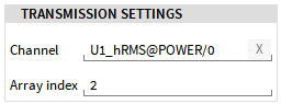
Fig. 385 Outputting arrays elements over CAN
Note that the preview will not show the currently transmitted data but has no functionality when the message mode is Transmit.
The Autonomous Resend option (see ① in Fig. 386) provides the following functionality for CAN buses which transmit data:
False (Default): The transceiver only sends the data once no matter if the receiver send an acknowledgement or not and sends the next message right afterwards. This makes the CAN da-ta transmission more deterministic on a correctly terminated CAN bus. But there is a remaining risk that a messages gets lost.
True: The risk of losing messages during transmission is low as message is resend in case no acknowledgement is sent by the receiver. But the risk of colliding messages of several transceivers is higher.
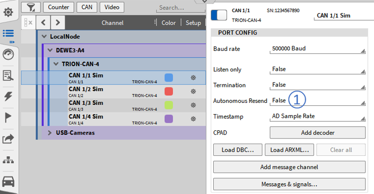
Fig. 386 Autonomous resend option
To tune the responsiveness and the signal quality of the transmitted data, we introduced the Out delay (see ③ in Fig. 384). This is the time, which the data is delayed before sent. The following graphs show the difference between two individual settings:
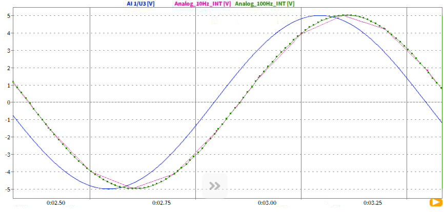
Fig. 387 Blue: Analog Input; Green: CAN-Output with a delay of 70 ms (default value)
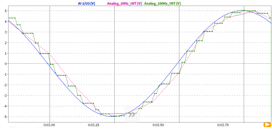
Fig. 388 Blue: Analog Input; Green: CAN-Output with a delay of 10ms
It is visible that a sample is repeated in case the delay is too low and no updated data is available yet.
Note
Message and Signal Encoding
The signals are encoded with the data type and length defined in the dbc-file or in the CAN sig-nal setup. If the channel has a value higher (or lower) than the possible range, the max (or min) value will be transferred. Make sure, you selected the right range and resolution for the specific channel not to lose information.
No channel assigned to a signal: the value 0 (Zero) is transmitted
Channel data is NaN: NaN is transmitted in case of float or double, 0 is transmitted in all other cases
For a better overview the reference channels for the CAN-Output will be listed in the channel list in the advanced section (see 19 in Fig. 175) with the column name “Reference channel” (see Fig. 389).
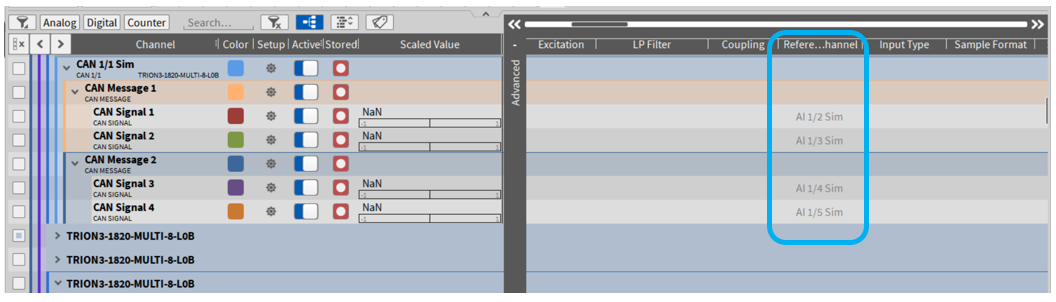
Fig. 389 CAN-OUT Reference channel
GPS channels
The following GPS data channels can be acquired by a TRION-TIMING or TRION-VGPS-20/-100 module:
Default channel name |
Channel mode |
Channel description |
Range |
Unit |
Data type |
Scaling available |
|---|---|---|---|---|---|---|
GPS |
NMEA |
GPS NMEA channel |
String |
x |
||
Latitude_GPS |
Latidtude |
Current latitude of the object |
-90° … 90° |
° |
Double |
✓ |
Longitude_GPS |
Longitude |
Current longitude of the object |
-180° … 180° |
° |
Double |
✓ |
Altitude_GPS |
Altitude |
Current altitude of the object |
-100 m … 1000 m |
m |
Double |
✓ |
Velocity_GPS |
Velocity |
Current velocity of the object |
0 km/h … 300 km/h |
km/h |
Double |
✓ |
Heading_GPS |
Direction |
Current heading of the object |
0° … 360° |
° |
Double |
✓ |
Satellites_GPS |
Sat |
Number of satellites in view |
0 … 24 |
Double |
x |
|
Fix Quality_GPS |
Quality |
GPS Fix |
String |
x |
||
H.Dilution_GPS |
HDOP |
2D deviation of longitude and latitude |
0 m … 100 m |
m |
Double |
✓ |
SoD_GPS |
Second |
Current second of the day |
0 s … 86400 s |
m |
Double |
x |
Date_GPS |
Date |
Current date in the format yyy-mm-dd hh:mm:ss:ms |
String |
x |
||
Acceleration_GPS |
Acceleration |
Current acceleration of the object |
-1000 m/s2… 1000 m/s2 … |
m/s2 |
Double |
✓ |
Distance_GPS |
Distance |
Distance covered from start of measurement |
0 m … 1000000 m |
m |
Double |
✓ |
Default channel name |
Acquired from TRION hardware |
Calculated channel |
Calculation |
|---|---|---|---|
GPS |
✓ |
x |
|
Latitude_GPS |
✓ |
x |
|
Longitude_GPS |
✓ |
x |
|
Altitude_GPS |
✓ |
x |
|
Velocity_GPS |
✓ |
x |
|
Heading_GPS |
✓ |
x |
|
Satellites_GPS |
✓ |
x |
|
Fix Quality_GPS |
✓ |
x |
|
H. Dilution_GPS |
✓ |
x |
|
SoD_GPS |
✓ |
x |
|
Date_GPS |
✓ |
x |
|
Acceleration_GPS |
x |
✓ |
Differentiation of channel Velocity_GPS |
Distance_GPS |
x |
✓ |
Integration of channel Velocity_GPS |
Note
The ranges of the channels are defined per default and have the purpose to define a min/max value if the channels are displayed in an Instrument. The ranges are neither minimum nor maximum limits. Thus, the defined ranges can be overrun and underrun without “clipping”.
Channels of data type double with physical unit can optionally be scaled (see ⑰ in Fig. 175). This option might be used for changing the physical channel unit from (kilo)meters to miles or km/h to mph.
Channels of data type double can be assigned to mathematical formulas (see Formula channel) or statistics calculations (see Statistics channel).
GPS channels cannot be filtered (see IIR Filter channel) as these channels are asynchronous channels.
During the measurement it might happen that the GPS Fix Quality is not fix all the time (i.e. GPS connection is lost during a ride through a tunnel). If this happens, the last value of the GPS channels will be hold until the GPS Fix Quality will be fix again and a new value is received.
If the GPS Fix Quality is not fix for more than 60 seconds, the calculated channels Acceleration_GPS and Distance_GPS will change to NaN until the GPS Fix Quality is fix again.
The GPS Fix Quality is fix if the channel receives 1 (GPS fix), 2 (Differential GPS fix), 3 (PPS fix), 4 (Real Time Kinematic) or 5 (Float RTK). The GPS Fix Quality is not fix if the channel receives 0 (Fix not available), 6 (Estimated (dead reckoning)), 7 (Manual input more) or 8 (Simulation mode)
The individual channels can be assigned to the following Instruments:
Default Channel Name |
GPS plot |
Analog Meter Digital Meter Bar Meter Indicator |
Recorder Chart Recorder |
Table |
Scope |
XY plot |
|---|---|---|---|---|---|---|
GPS* |
x |
x |
x |
✓ |
x |
x |
Latitude_GPS |
✓ |
✓ |
✓ |
✓ |
✓ |
✓ |
Longitude_GPS |
✓ |
✓ |
✓ |
✓ |
✓ |
✓ |
Altitude_GPS |
x |
✓ |
✓ |
✓ |
✓ |
✓ |
Velocity_GPS |
x |
✓ |
✓ |
✓ |
✓ |
✓ |
Heading_GPS |
✓ |
✓ |
✓ |
✓ |
✓ |
✓ |
Satellites_GPS |
x |
✓ |
✓ |
✓ |
✓ |
✓ |
Fix Quality_GPS |
x |
x |
x |
x |
x |
x |
H.Dilution_GPS |
x |
✓ |
✓ |
✓ |
✓ |
✓ |
SoD_GPS |
x |
✓ |
✓ |
✓ |
✓ |
✓ |
Date_GPS |
x |
x |
x |
x |
x |
x |
Acceleration_GPS |
x |
✓ |
✓ |
✓ |
✓ |
✓ |
Distance_GPS |
x |
✓ |
✓ |
✓ |
✓ |
✓ |
*The channel GPS can be dragged and dropped directly from the Channel List to the measurement screen. If this is performed, the current value of the channels Latitude, Longitude, Altitude, Velocity, Heading, Satellites used, Quality and Dilution will be displayed (see Fig. 390).
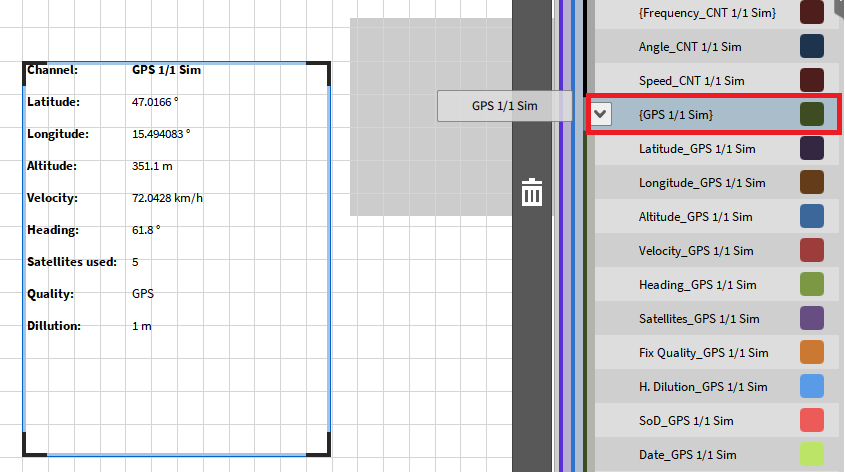
Fig. 390 Drag and drop the GPS channel to the measurement screen
Note
During GPS-channel analysis in PLAY mode, the GPS channels can also be exported to *.txt, *.csv, *.mdf4 or *.mat format (see Export Settings). Please note that GPS-Channels of data type String can only be exported to *.txt or *.csv format as the data type is not supported for *.mdf4 and *.mat format.
TEDS support
TEDS stands for Transducer Electronic Datasheet and is used to identify and apply settings from a sensor directly without manually entering them. The following TRION(3) modules support TEDS:
TRION(3)-18xx-MULTI
TRION-2402-MULTI
TRION-2402-dACC1
1TEDS functionality only supported in IEPE® mode.
Use in OXYGEN
If a sensor with TEDS interface is connected to an according TRION(3) module, the TEDS interface is automatically detected and the settings are applied to the channel.
To scan for a TEDS interface, also on multiple channels, there is a button Scan TEDS on the lower edge of the channel list menu, seen in Fig. 391. Whenever the full channel list menu is open, the scan for TEDS is done continuously and a manual scan is not necessary when the sensor is changed. This is not the case for the TRION-2402-dACC, where the scan must be done with the button in order to scan for TEDS.
It is also possible to disable the TEDS detection by choosing one or multiple channels in the channel list and clicking on the button Disable TEDS, also seen in Fig. 391. After disabling the TEDS detection, all set settings from the TEDS are deleted and can be entered manually.
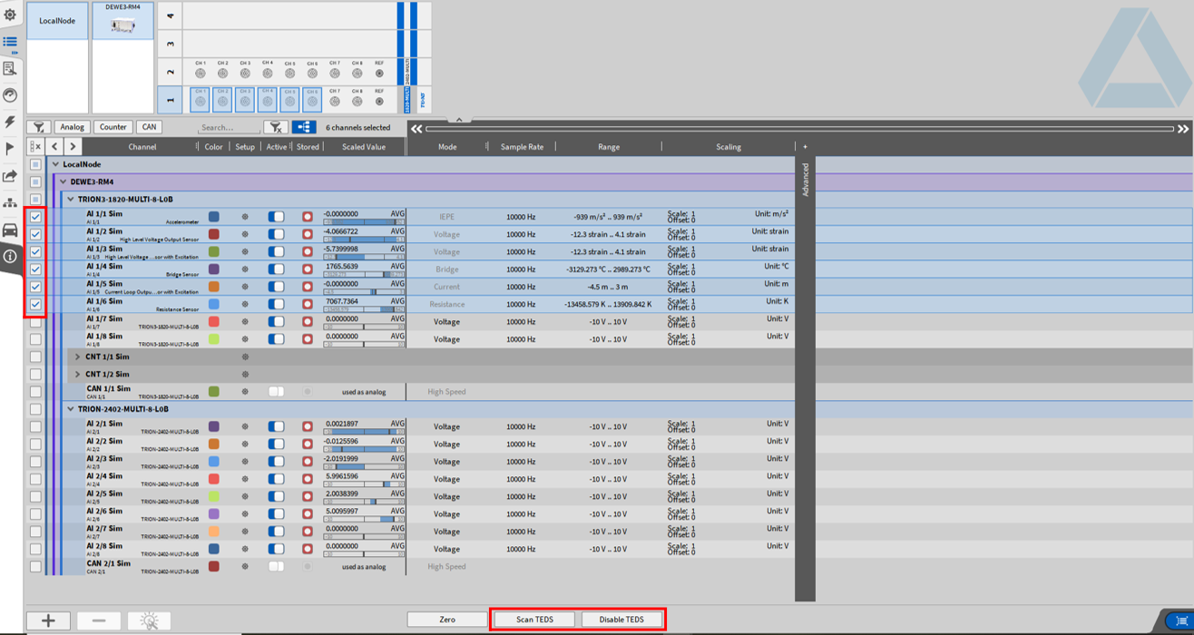
Fig. 391 Channel List Menu and TEDS scanning
A detailed channel setting can be seen in Fig. 392. Depending on the type of sensor some settings might vary. The settings from the TEDS can be seen here and some settings can be adjusted manually, like the range. By clicking on the shown TEDS serial number, marked red in Fig. 392, all the TEDS information and settings can be seen (see blue frame in Fig. 392).
By clicking on “Editor” (see green circle in Fig. 392) the TEDS editor can be opened (see green frame) which offers the possibility to edit the stored data on the TEDS chip. It is possible to choose between a set of templates (see ① in Fig. 392) or to change the information stored on the TEDS chip manually (see ② in Fig. 392). When all changes are finished the information can be written to the TEDS chip, by clicking on “Write to TEDS” (see purple circle in Fig. 392). A window will pop up which asks for confirmation that the data should be written to the TEDS chip.
Note
If the changes will be stored on the TEDS chip, the existing data on the TEDS chip gets lost.
The following TEDS chips are supported: - DS2406 - DS2430A - DS2431 - DS2432 - DS2433
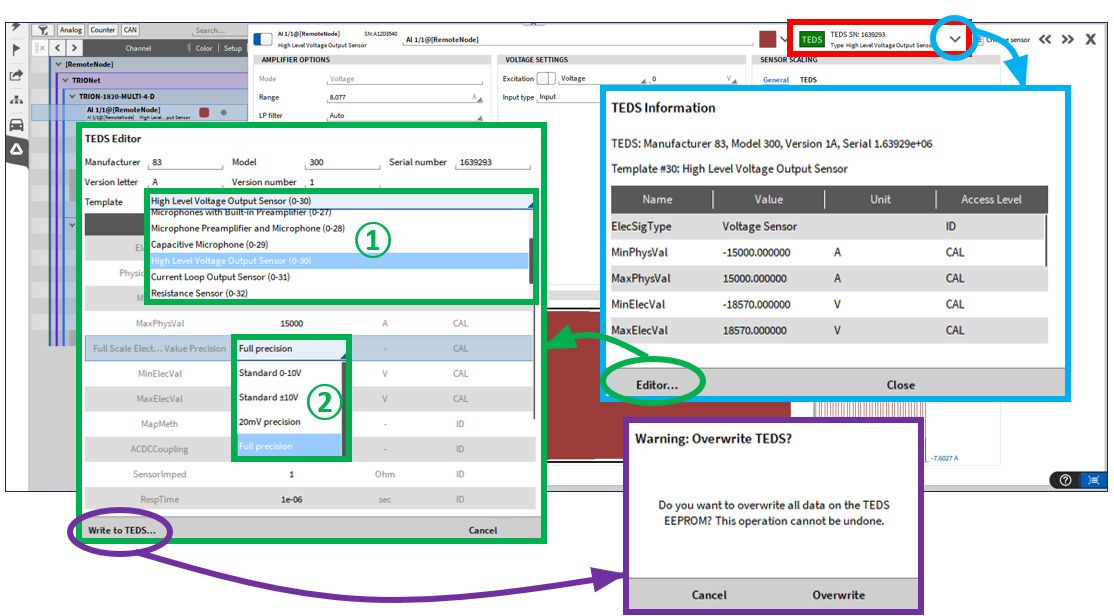
Fig. 392 Detailed Channel Settings with TEDS interface and TEDS editor
To prevent the TEDS data from being overwritten by mistake, the function for writing TEDS chips is deactivated by default. To activate the function, go to the Advanced settings in the OXYGEN Setup and activate the corresponding checkbox “Enable TEDS editor” (see Fig. 393).
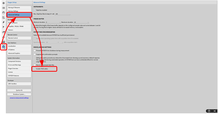
Fig. 393 Activation for writing data to TEDS
More information about the set scaling can be found in the Sensor Scaling section by switching to the TEDS tab. This cannot be changed and is only for information for the user. However, it is possible to add an additional scaling in the General tab, which will be used additionally to the already set scaling from the TEDS.
More information about the set scaling can be found in the Sensor Scaling section by switching to the TEDS tab. The current scaling will be written in grey and cannot be changed directly and is only for information for the user. To change the scaling information it is possible to perform a 2-point scaling (for detailed information see “Changing the 2-point-scaling” in Changing the channel settings) and write it to the TEDS chip by clicking “Write to TEDS in the scaling section of the channel settings (see Fig. 394).
Note
If the changes are stored on the TEDS chip, the existing data on the TEDS chip gets lost. However, it is possible to add an additional scaling in the General tab, which will be used additionally to the already set scaling from the TEDS.
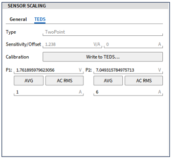
Fig. 394 Sensor Scaling Information: TEDS
TEDS detection can also be disabled in the detailed settings by clicking on the green TEDS button (marked green in Fig. 392). This button has different colors depending on the state, which will be explained here:
 TEDS active; sensor was detected and is in use.
 TEDS active; no sensor was detected.
 TEDS active; sensor was detected but is not compatible, remove the sensor or disable TEDS.
This case is also shown in the channel list:

 TEDS active, sensor lost and not detected anymore
 TEDS disabled
Loading a setup
When loading a setup, OXYGEN automatically checks the if the same TEDS can be detected on the current system. If there is a mismatch in the TEDS detection, this specific channel or rather TEDS type is marked red. If a new sensor is detected, the new detected TEDS will be marked red, seen in Fig. 395 and the new settings of the sensor can be applied by clicking on Apply of the pop-up window. Otherwise, the remapping must be cleared and the channels, on which the settings should be applied, must be remapped manually, seen in Fig. 396. If a sensor from the setup file is missing and is not detected when loading the file, the TEDS type will show the message missing, seen in Fig. 397.
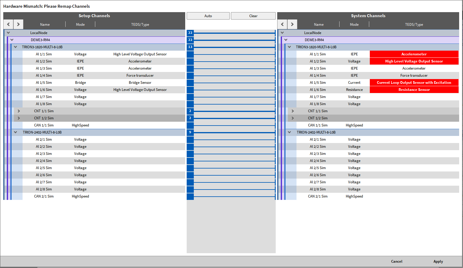
Fig. 395 Hardware mismatch: different TEDS were detected
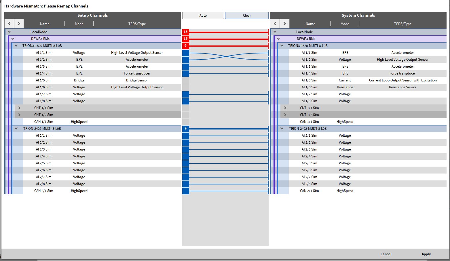
Fig. 396 Hardware mismatch: manual remapping of TEDS
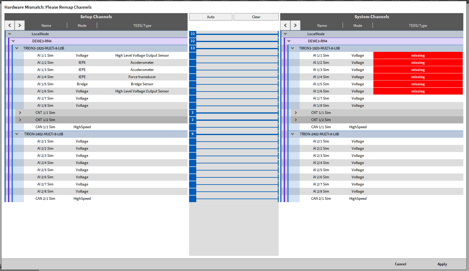
Fig. 397 Hardware mismatch: missing TEDS in loaded setup file