d/q Analysis (OPT-POWER-ADV)
This chapter describes the d/q analysis feature. The d/q analysis can be performed with a mechanical angle signal and sensorless without the need of an angle signal. The sensorless calculation requires specification of stator resistance and stator inductance The d/q analysis is designed for use with 3-phase synchronous machines.
The d/q transformation is also known as Park-Clarke transformation, often used in field orientated control to get steady state feedback of the machines current and flux. To perform the analysis with mechanical angle, any kind of angle signal (rotor position) must be provided.
Measured Angle
Following settings are for the d/q analysis with mechanical angle input.
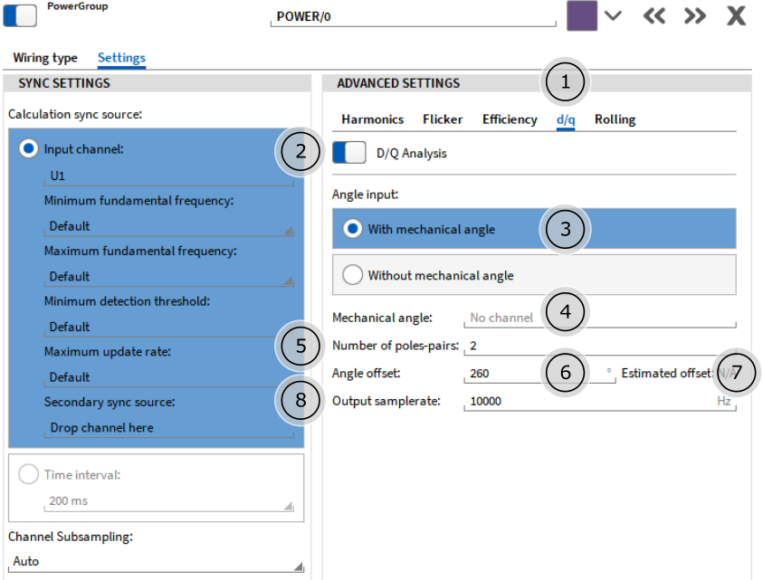
Fig. 56 Detail Settings in OXYGEN Power Group
Details Tab for Settings of the d/q analysis
Enable/Disable d/q calculation
Angle input selection, calculation with mechanical angle is selected
Input field for mechanical angle channel (drag-n-drop), must provide an angle signal between 0-360 deg.
Input field for number of pole-pairs
Input field for offset of the mechanical angle to the electrical (deg)
Button to detect the actual angle offset (use only without load)
Channel Output Sample rate (100 Hz is default).
Estimated Angle
Following settings are for the d/q analysis without mechanical angle input.
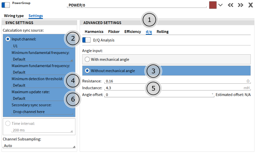
Fig. 57 Detail Settings in OXYGEN Power Group
Details Tab for Settings of the d/q analysis
Enable/Disable d/q calculation
Angle input selection, calculation without mechanical angle is selected
Input field for stator resistance (Ohm)
Input field for stator inductance (mH)
Input field for offset of the electrical angle to exact d-axis alignment (deg). This is just a debug channel and can be kept at zero.
The sensorless d/q computes the rotor posistion by calculating the electromotoric force (EMF) of the synchronous machine under use of stator resistance and inductance. This calculation assumes electric and magnetic symmetry and uniformity in all orientations. Since EMF is bound to the change of the magnetic field an thus the speed of the machine, the accuracy of the sensorless calculation suffers at low speeds. Acceptable results are achieved for speeds above 5% of nominal speed ( ).
).
The calculated angle of the sensorless computation can be found in the “dq_angle” channel of the d/q analysis. Unlike the calculation with mechanical angle input the sensorless version does not have a fixed output rate. It calculates 100 samples per electrical period and is therefore inherently asychronous, just like the power group. The following quick start guide is intended for the d/q analysis with mechanical angle input.
Quick Start
The key to get accurate readings from the resulting d/q channels is a good alignment of the Rotor Axis to the angle measurement sensor. To support the user with this task, we implemented a semi-automatic workflow.
Prepare the Typical power group settings for power analysis
Enable the d/q analysis feature (only possible within 3-phase measurements)
Assign the angle channel
Edit the number of pole-pairs according to your engine
Drive the DUT (device under test) with an auxiliary engine at constant speed (idle)
Press the “Detect” Button
Check the detected value
If there is no possibility to run the engine with an auxiliary drive, there are two other methods:
Use the moment of inertia and use the induced voltage during coast down
Drive your engine without any load at slow speed e.g. 100 rpm to reduce the effects of friction and ventilation
Angle Measurement
There are different methods available to measure the actual rotor position, these are necessary for the d/q analysis with mechanical angle:
Rotary Encoder
The rotary encoder is typically used in slow to medium speed drives. The signal of this encoders can be processed by the following Hardware inputs and transformed to an angle signal:
TRION-CNT
TRION-Base
TRION-Timing / VGPS
TRION-1802-dLV
One Pulse per Turn
In the case, where there no option to mount a rotary encoder, a single impulse (Z) can also be used as source for the angle measurement (with the same hardware listed above). The single pulse can be generated by a inductive or laser sensor.
SIN/COS Sensors
If your engine is equipped with an SIN/COS sensor (Magnetic field sensor, XMR-Sensor), use an analog input for these two signals. To calculate the correct angle, please create the following formula in OXYGEN: 
Channel Reference
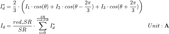
The channel reference reveals how the d/q analysis output channels are calculated. Note that the variant with mechanical angle input uses raw waveforms channels for voltage and current and the sensorless method uses the fundamental counterparts.
Symbol |
Equation |
Description |
|---|---|---|
|
|
Actual rotor angle |
|
– |
Samplerate of U/I Channels |
|
– |
Reduced Samplerate for Output |
|
– |
Line-to-Neutral Voltage of Phase i |




U_d
d-Axis Voltage, reduced with block-wise average to given output samplerate.

U_q
q-Axis Voltage, reduced with block-wise average to given output samplerate.

I_d
d-Axis Current, reduced with block-wise average to given output samplerate.
I_q
q-Axis Current, reduced with block-wise average to given output samplerate.
