Rolling Computation (OPT-POWER-EXP)
This chapter describes the Rolling Computation feature. It is designed for analysing fast changes in power grid connected applications e.g. renewable energy testing. In advance to the “normal” calculation, which is performed each single fundamental period, the computation in default setting is done every 1ms over the period of one fundamental cycle.
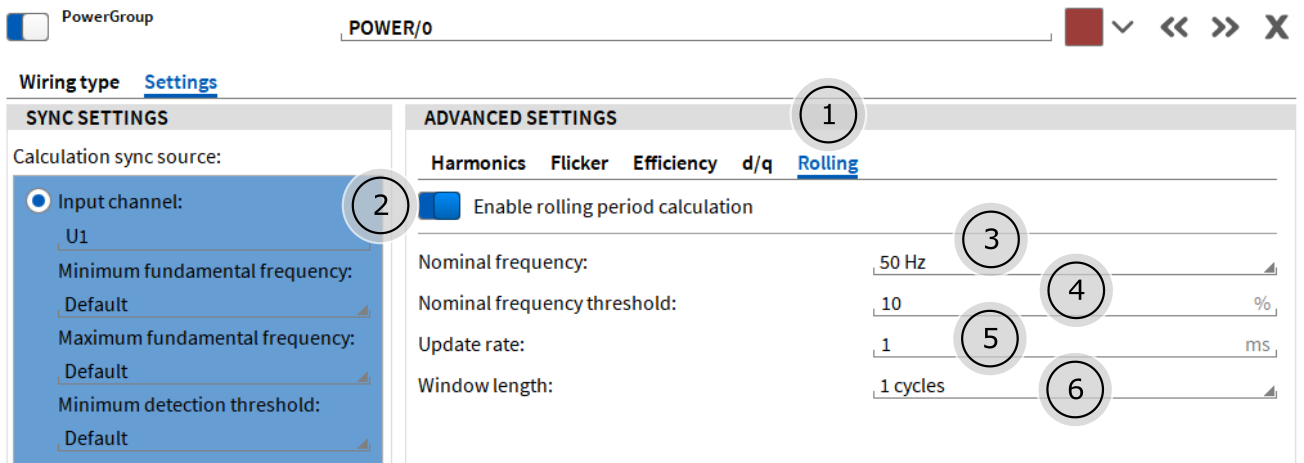
Fig. 53 Detail Settings in OXYGEN Power Group
Details Tab for Settings of the rolling computation
Enable/Disable Rolling Calculation
Selector for nominal frequency fallback (50 Hz / 60 Hz)
Input field for frequency threshold.
If a frequency is detected within the nominal frequency
 threshold %, the rolling window size is the actual period duration. Otherwise, e.g. in the case of a voltage interruption, where no frequency can be measured, the window size is the inverse nominal frequency (0–95 %).
Update rate (0.1–20 ms)
Window length (0.5 cycles / 1 cycles)
Attention
The following graph shows the details of the operation principle. It is similar to a moving average calculation, but with a variable window size, which depends on the actual measured fundamental frequency. If the calculate window size exceeds the maximum allowed size, which is given by (1/Nominal Frequency)*(1 + Frequency Threshold/100), the window size is set to 1/Nominal Frequency.
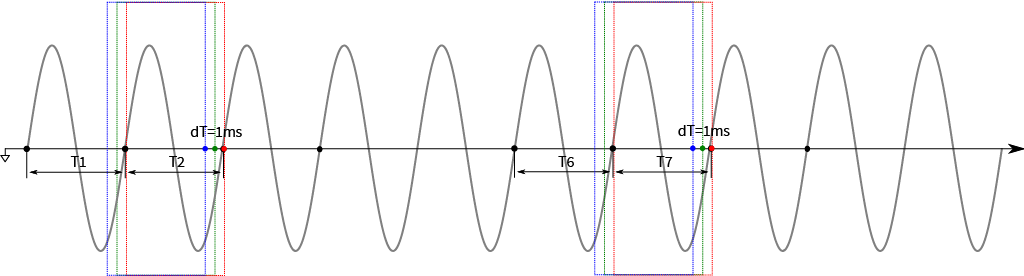
Fig. 54 Detail Settings in OXYGEN Power Group
Channel Reference (Basic)
Some of the shown intermediate results or variables are not available in the software today. They are marked with a *.
Symbol |
Equatiom |
Description |
|---|---|---|
|
– |
Samplerate |
|
– |
Number of Power Phases |
|
|
Number of Samples |


U[i]_tRMS_rc
This is the Power Phase number i True RMS Voltage, updated every 1ms.
![\begin{aligned}
U[i]_{tRMS\_rc} &= \sqrt{\frac{1}{N} \sum_{n=0}^{N} u_i[n]^2} & Unit: \mathbf{V}
\end{aligned}](../_images/math/7796fd9811c08530aa2d0e208fd53d9e7aeac8ef.png)
U[ij]_tRMS_rc
This is the Line-Line ij True RMS Voltage, updated every 1ms. This channel is only available in 3-Phase Power Configurations.
![\begin{aligned}
U[ij]_{tRMS\_rc} &= \sqrt{\frac{1}{N} \sum_{n=0}^{N} \left( u_i[n]-u_j[n] \right) ^2} & Unit: \mathbf{V}
\end{aligned}](../_images/math/a197d9b969c1b738bca06998d92418df960a806f.png)
I[i]_tRMS_rc
This is the Power Phase number i True RMS Current, updated every 1ms.
![\begin{aligned}
I[i]_{tRMS\_rc} &= \sqrt{\frac{1}{N} \sum_{n=0}^{N} i_i[n]^2} & Unit: \mathbf{A}
\end{aligned}](../_images/math/8f5bbc963ece7d21194cf9a736b1303448337c14.png)
P_t_rc
This is the Power Group Overall active Power, updated every 1ms.
![\begin{aligned}
P_{t\_rc} &= \sum_{i=1}^{NP} P[i]_{t} & Unit: \mathbf{W}
\end{aligned}](../_images/math/ef34433c683b5a64799c4f1ed3cf0db91e76d7fe.png)
P[i]_t_rc
This is the Power Phase number i active Power, updated every 1ms.
![\begin{aligned}
P[i]_{t\_rc} &= \frac{1}{N} \sum_{n=0}^{N} u_i[n] \cdot i_i[n] & Unit: \mathbf{W}
\end{aligned}](../_images/math/5f7f384842e3bb019f1eb6707395575a794af62b.png)
P_fund_rc
This is the Power Group Overall fundamental active Power, updated every 1ms.
![\begin{aligned}
P_{fund\_rc} &= \sum_{i=1}^{NP} P[i]_{fund\_rc} & Unit: \mathbf{W}
\end{aligned}](../_images/math/4d9a53c1cb0b840e9a383cd86018f745ddfe5a6d.png)
P[i]_fund_rc
This is the Power Phase number i fundamental active Power, updated every 1 ms.
![\begin{aligned}
P[i]_{fund\_rc} &= U[i]_{fundRMS\_rc} \cdot I[i]_{fundRMS\_rc} \cdot cos \left( P[i]_{fundPHI\_rc} \right) & Unit: \mathbf{W}
\end{aligned}](../_images/math/be34951b62afbc797cb2d05b1eaccfb2497bf863.png)
![U[i]_{fundRMS\_rc} , P[i]_{fundPHI\_rc}](../_images/math/2be5c2a3d063909128a5af2abfd8f78223479f2e.png) are internal channels, not available for users.
are internal channels, not available for users.
Q_t_rc
This is the Power Group Overall reactive Power, updated every 1ms.

Q[i]_t_rc
This is the Power Phase number i reactive Power, updated every 1 ms.
![\begin{aligned}
Q[i]_{t\_rc} &= s \cdot \sqrt{S[i]_{t\_rc}^2 - P[i]_{t\_rc}^2} \hspace{3em} s =
\begin{cases}
1 & \quad \text{if } Q_{fund\_rc} > 0\\
-1 & \quad \text{if } Q_{fund\_rc} <= 0\\
\end{cases}
& Unit: \mathbf{var}
\end{aligned}](../_images/math/438b36ac271d276f8304339a18dd2ba479e519ea.png)
Q_fund_rc
This is the Power Group Overall fundamental reactive Power, updated every 1ms.
![\begin{aligned}
Q_{fund\_rc} &= \sum_{i=1}^{NP} Q[i]_{fund\_rc} & Unit: \mathbf{var}
\end{aligned}](../_images/math/158f3022e09201991478643e7a19c7264e4db554.png)
Q[i]_fund_rc
This is the Power Phase number i fundamental reactive Power, updated every 1ms.
![\begin{aligned}
Q[i]_{fund\_rc} &= U[i]_{fundRMS\_rc} \cdot I[i]_{fundRMS\_rc} \cdot sin \left( P[i]_{fundPHI\_rc} \right) & Unit: \mathbf{var}
\end{aligned}](../_images/math/2a2ec266224f34fe4646e05fea8cacf27bf031d0.png)
S_t_rc
This is the Power Group Overall apparent Power, updated every 1ms.
![\begin{aligned}
S_{t\_rc} &= \sum_{i=1}^{NP} S[i]_{t\_rc} & Unit: \mathbf{VA}
\end{aligned}](../_images/math/9283c3f1c3f0af279a730e3e84b14d564aa924c6.png)
S[i]_t_rc
This is the Power Phase number i apparent Power, updated every 1ms.
![\begin{aligned}
S[i]_{t\_rc} &= U[i]_{tRMS\_rc} \cdot I[i]_{tRMS\_rc} & Unit: \mathbf{VA}
\end{aligned}](../_images/math/dfd64db943707f82f217bb95098d637492430276.png)
S_fund_rc
This is the Power Group Overall fundamental apparent Power, updated every 1ms.
![\begin{aligned}
S_{fund\_rc} &= \sum_{i=1}^{NP} S[i]_{fund\_rc} & Unit: \mathbf{VA}
\end{aligned}](../_images/math/c95c4ea704df395e7b957f456b506dbd504b9e15.png)
S[i]_fund_rc
This is the Power Phase number i fundamental apparent Power, updated every 1ms.
![\begin{aligned}
S[i]_{fund\_rc} &= U[i]_{fundRMS\_rc} \cdot I[i]_{fundRMS\_rc} & Unit: \mathbf{VA}
\end{aligned}](../_images/math/e4c5385ca400039439a477805146135f050ab15e.png)
U_DC_rc
This is the DC Voltage in case the DC Power Analysis is enabled in the Efficiency tab, updated every 1ms.
![\begin{aligned}
U_{DC\_rc} &= \frac{1}{N} \sum_{n=0}^{N} u_{DC}[n] & Unit: \mathbf{V}
\end{aligned}](../_images/math/0bacb34f9f4d4e526382b01ef80b1ba472b10295.png)
I_DC_rc
This is the DC Current in case the DC Power Analysis is enabled in the Efficiency tab, updated every 1ms.
![\begin{aligned}
I_{DC\_rc} &= \frac{1}{N} \sum_{n=0}^{N} i_{DC}[n] & Unit: \mathbf{A}
\end{aligned}](../_images/math/c5249c924dc3cc0a18c2344aa7dd23fc97f9cdbb.png)
P_DC_rc
This is the DC Power in case the DC Power Analysis is enabled in the Efficiency tab, updated every 1ms.
![\begin{aligned}
P_{DC\_rc} &= \frac{1}{N} \sum_{n=0}^{N} u_{DC}[n] \cdot i_{DC}[n] & Unit: \mathbf{W}
\end{aligned}](../_images/math/02cee6d0c5a87a153ed6d6800d0554429d0bdddc.png)
Channel Reference (Symmetrical Components)
This section describes the equations for symmetrical components according to FGW-TG3 Annex F and IEC 61400-21 Annex C.
U[i]_fund_cos_rc
This is the Real part of the fourier coefficients of the signal. (F-1 in FGW-TG3 Annex F)
![\begin{aligned}
U[i]_{fund\_cos\_rc} & = \frac{2}{N} \sum_{n=-N-1}^{0} u_i[n] \cdot cos(2\cdot\pi \cdot F_{fund} \cdot \frac{n}{SR}) & Unit: \mathbf{V}
\end{aligned}](../_images/math/bc24f1f7a8ed6eba4992f18fa269ce90bbe92c27.png)
U[i]_fund_sin_rc
This is the Imaginary part of the fourier coefficients of the signal (F-2 in FGW-TG3 Annex F).
![\begin{aligned}
U[i]_{fund\_sin\_rc} & = \frac{2}{N} \sum_{n=-N-1}^{0} u_i[n] \cdot sin(2\cdot\pi \cdot F_{fund} \cdot \frac{n}{SR}) & Unit: \mathbf{V}
\end{aligned}](../_images/math/e35b311ed1c68dcd4b1c322c471fa78c38dcdb10.png)
U_fundCOS_SYM+_rc
This is the real vector component of the Positive Voltage Sequence.

U_fundSIN_SYM+_rc
This is the imaginary vector component of the Positive Voltage Sequence.

U_fundPHI_SYM+_rc
This is the phase angle of the Positive Voltage Sequence.

U_fundCOS_SYM-_rc
This is the real vector component of the Negative Voltage Sequence.

U_fundSIN_SYM-_rc
This is the imaginary vector component of the Negative Voltage Sequence.

U_fundPHI_SYM-_rc
This is the phase angle of the Negative Voltage Sequence.

U_fundCOS_SYM0_rc
This is the real vector component of the Zero Voltage Sequence.

U_fundSIN_SYM0_rc
This is the real vector component of the Zero Voltage Sequence.

U_fund_SYM+_rc
This is the RMS value of the Phase-Phase (Line-Line) voltages positive sequence system.

U_fund_SYM-_rc
This is the RMS value of the Phase-Phase (Line-Line) voltages negative sequence system.

U_fund_SYM0_rc
This is the RMS value of the Phase-Phase (Line-Line) voltages zero sequence system.

I[i]_fund_cos_rc
This is the Real part of the fourier coefficients of the signal (F-1 in FGW-TG3 Annex F).
![\begin{aligned}
I[i]_{fund\_cos\_rc} & = \frac{2}{N} \sum_{n=-N-1}^{0} I_i[n] \cdot cos(2\cdot\pi \cdot F_{fund} \cdot \frac{n}{SR}) & Unit: \mathbf{A}
\end{aligned}](../_images/math/af6a20eafa778bba90d9d781b8915c101a6705b3.png)
I[i]_fund_sin_rc
This is the Imaginary part of the fourier coefficients of the signal. (F-2 in FGW-TG3 Annex F)
![\begin{aligned}
I[i]_{fund\_sin\_rc} & = \frac{2}{N} \sum_{n=-N-1}^{0} I_i[n] \cdot sin(2\cdot\pi \cdot F_{fund} \cdot \frac{n}{SR}) & Unit: \mathbf{A}
\end{aligned}](../_images/math/34361feeb3f9563635314d9f3668deed1d4a8361.png)
I_fundCOS_SYM+_rc
This is the real vector component of the Positive Current Sequence.

I_fundSIN_SYM+_rc
This is the imaginary vector component of the Positive Current Sequence.

I_fundCOS_SYM-_rc
This is the real vector component of the Negative Current Sequence.

I_fundSIN_SYM-_rc
This is the imaginary vector component of the Negative Current Sequence.

I_fundCOS_SYM0_rc
This is the real vector component of the Zero Current Sequence.

I_fundSIN_SYM0_rc
This is the real vector component of the Zero Current Sequence.

P_fund_SYM+_rc

P_fund_SYM-_rc

P_fund_SYM0_rc

Q_fund_SYM+_rc

Q_fund_SYM-_rc

Q_fund_SYM0_rc

S_fund_SYM+_rc

S_fund_SYM-_rc

S_fund_SYM0_rc

I_fund_P_SYM+_rc

I_fund_P_SYM-_rc

I_fund_P_SYM0_rc

I_fund_Q_SYM+_rc

I_fund_Q_SYM-_rc

I_fund_Q_SYM0_rc

PF_fund_SYM+_rc

PF_fund_SYM-_rc

PF_fund_SYM0_rc
