Technical Calculation Remarks

The following section includes important hints for the calculation methods referring to the output channels of the order analysis module.

Sample Rate

• Recommendation for minimum sample rate:

Example: Maximum Speed = 6000 rpm / 60 * 100 * 3 = 30 kS/s Highest Order: 100

Speed Range

• Minimum speed: 60 rpm

• Maximum speed: 100 000 rpm

• Possible range from minimum to maximum speed: 2 decades (i.e. from 100 to 10000 rpm)

• Speed resolution: up to 1000 speed steps

• The speed resolution is limited to 1000 steps (and therefore both the order and the fre-quency matrix are limited to 1000 lines).

• This was done to avoid RAM overload and to ensure proper data handling for post pro-cessing in 3rd party SW packages.

• Speed intervals: Calculation and sorting of speed values in different intervals

• Depending on the settings for Minimum speed, Maximum speed and Speed resolution, the speed is split into the following intervals (This applies for the speed resolution of the order and the frequency spectrum):

Interval	Label / Interval name	Lower boundary (included)	Upper boundary (excluded)
Interval 1	ceil(min_speed / speed_resolution) * speed_resolution	min_speed	Label + speed_resolution/2
Interval 2	Interval 1 + speed_resolution	Label - speed_resolution/2	Label + speed_resolution/2
Interval 3	Interval 2 + speed_resolution	Label - speed_resolution/2	Label + speed_resolution/2
…	…	…	…
Interval k	floor(max_speed / speed_resolution) * speed_resolution	Label - speed_resolution/2	max_speed

• Example1: min_speed = 60, max_speed = 6000, speed_resolution = 100

Interval 1	100	60	150
Interval 2	200	150	250
Interval 3	300	250	350
…	…	…	…
Interval k	5900	5850	6000

• If a certain speed interval is not passed during the run up or the coast down of the engine was too fast, the data between the measured upper and lower interval will be linear interpo-lated to fill the interval gaps with data.

• Example:

Interval	Label / Interval name	Data determined	Data displayed
Interval 1	100	Yes	Determined
Interval 2	200	Yes	Determined
Interval 3	300	No	Interpolated between 200 and 400 rpm
Interval 4	400	Yes	Determined
Interval 5	500	No	Interpolated between 400 and 600 rpm
Interval 6	600	Yes	Determined
Interval 7	700	No	Interpolated between 600 and 900 rpm
Interval 8	800	No	Interpolated between 600 and 900 rpm
Interval 9	900	Yes	Determined

Frequency and Order Matrices

Both the frequency matrix and the order matrix are calculated in 2 parallel stages. The frequency ma-trix is calculated using a standard FFT algorithm to transform the time signal in fixed intervals (2n) into the frequency domain and the order matrix is calculated based on a FFT transforming the time signal per every revolution into the frequency domain. More details can be found in the following sections.

The frequency and order matrices contain no time dependent data. This means that the matrices are filled continuously with data while the measurement is running but the data will be stored without timestamping. When the data is analyzed in PLAY mode the content of the matrix will not change but remain in the same manner as at the end of the measurement.

If the same speed step is passed several times during the measurement, only the maximum value will be stored to each matrix column. Minor values will be overwritten and not stored to the data file.

Determination of the Frequency Matrix

• The FFT size depends on the minimum and maximum speed and the order resolution.

• The maximum FFT size in samples is limited to 4096. This leads to a maximum number of 2048 FFT bins in the frequency matrix.

• The limited number of 2048 FFT bins (and therefore 2048 matrix columns from 0 Hz to Hz) was done to avoid RAM overload and to ensure proper data handling for post processing in 3rd party SW packages.

• The user can select between the following window functions for the FFT determination:

• Hamming (default), Hanning, Rectangular, Blackman, Blackman-Harris, Flat-top, Bartlett (Tri-angular)

• Choose an overlapping factor in time domain of 0%, 50%, 75%, 80% and 90%

Determination of the Order Matrix

General:

• The order resolution can be set from 0.01 to 1.

• The maximum order depends on the order resolution. The maximum number of columns for the order matrix is 2048 to avoid RAM overload and to ensure proper data handling for post processing in 3rd party SW packages.

• The maximum order is displayed at the bottom of the Generic options of the order analysis setup.

• If the order resolution is not specified as an inverse integer multiple of 1, the order resolu-tion will be rounded automatically to the next lower inverse integer multiple of 1.

• I.e. 0.4 will be rounded to 1/3, 0.6 will be rounded to 0.5

The calculation steps from the raw input signal in time domain to the order matrix are the following:

• Separation of the raw input signal into signal blocks per revolution (see Fig. 19 top); One block represents one revolution; to achieve a high accuracy, the rotation angle is required therefore.

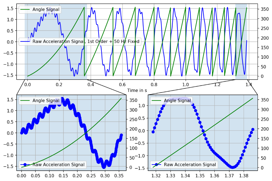
Fig. 19 Separation into separate blocks per revolution (top); Decreasing number od samples with increasing running speed (bottom)

As the running speed of the DUT will change continuously and the sample rate is constant , the number of samples per revolution will decrease with increasing running speed (see Fig. 19 bottom).

• The average speed per revolution is determined and stored to the Speed channel which is output by the order analysis module

• To avoid aliasing during the FFT explained in the following below, the raw signal will be fil-tered with an adaptive anti-aliasing filter (lowpass filter) (see section Fig. 20).

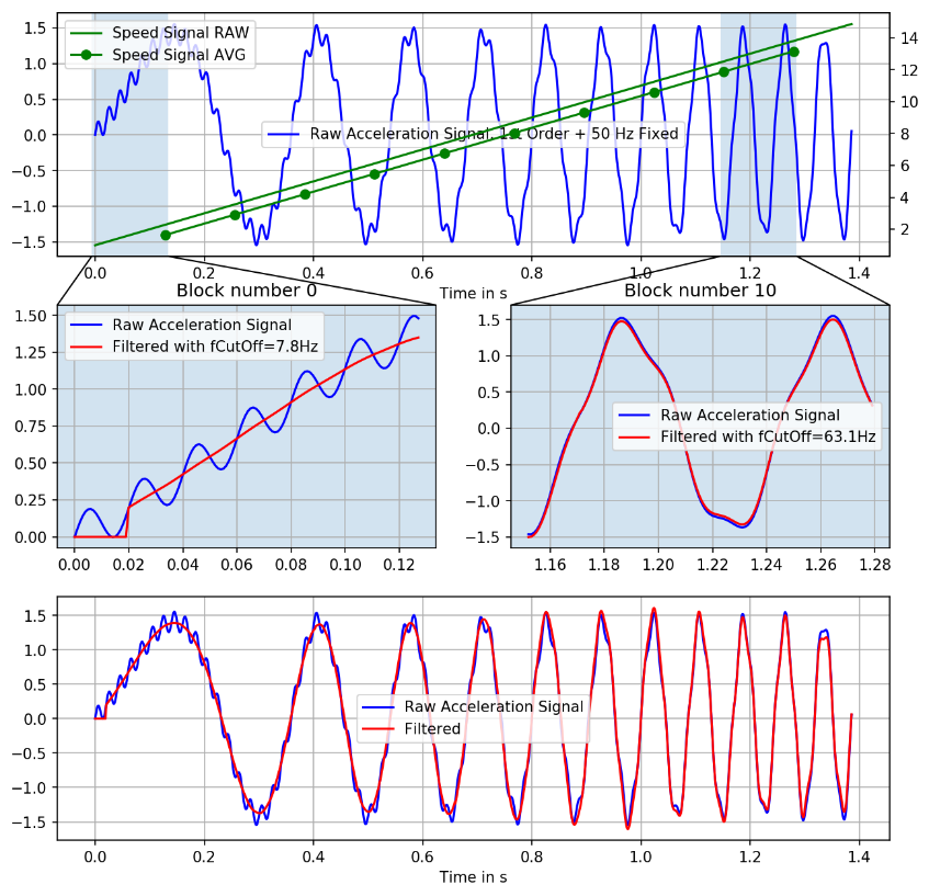
Fig. 20 Impact of the anti-aliasing filter to the raw signal

• Due to the fact mentioned above that the numbers of samples per revolution is decreasing with increasing running speed, the signal will be resampled to a defined number of samples per revolution (see Fig. 21).

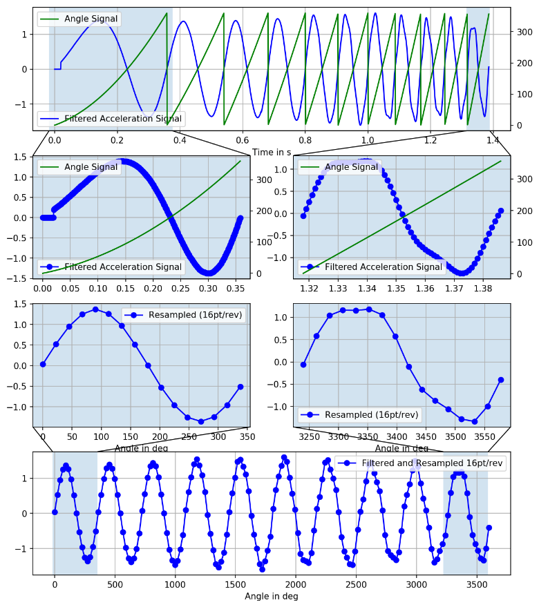
Fig. 21 Resampling to a defined number of samples per revolution

An accurate angle signal is required for this step. The more angle steps per revolution delivered by the speed sensor, the more accurate the resampling algorithm will work. This means that an encoder de-livering 1800 pulses per revolution will lead to more accurate results than an encoder delivering 512 pulses per revolution as the angle resolution is better.

A linear interpolation algorithm is used for resampling.

The number of samples per revolution depends on the sample rate and the maximum speed.

• The order spectrum is now calculated by transforming the resampled signal (fixed number of samples per revolution) into the frequency domain.

• The difference to the output spectrum to the usual frequency spectrum is hereby that the frequency is no longer plotted along the x-axis but the order itself (see Fig. 22). Thus, the order spectrum can be directly extracted from this spectrum.

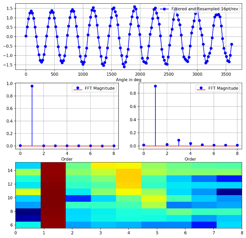
Fig. 22 Determination of the order spectrum

Note

• The Overlapping factor specified in the Frequency spectrum options of the order analysis set-tings is also applied to the order spectrum.

• The Window function specified in the Frequency spectrum options of the order analysis set-tings is not applied to the order spectrum but only to the frequency spectrum.

Extraction of Orders from Intensity Diagram

It is possible to extract the order from an intensity diagram via the cursor position (see Fig. 23). To enable the order extraction, press the icon on the upper right corner of the intensity diagram (①) and move the cursor in the diagram to the desired order. The size of the order extraction can be expanded by dragging the grey bar between the two diagrams. For better visualization, enable logarithmic scal-ing.

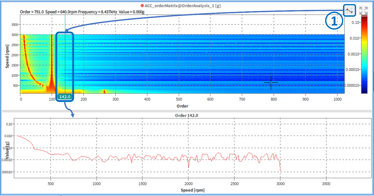
Fig. 23 Extraction of order from intensity diagram