Understanding Modal Test
This chapter describes the calculation princeples and recorded data channels.
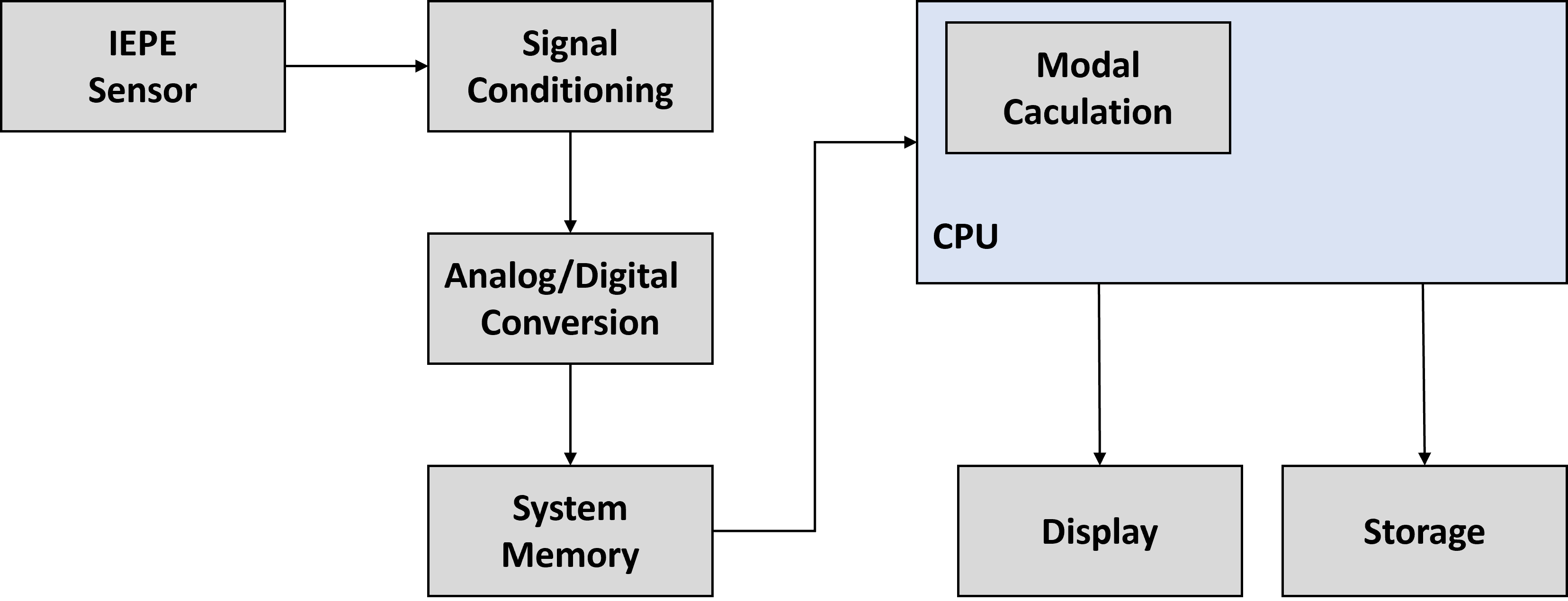
Fig. 24 Signal and Data flow
Calculation modes
In this chapter, the calculation modes for all relevant results will be explained.
FRF - Frequency Response function
The FRF is calculated between each excitation/response pair in mono or triaxial mode, depending on the sensor. These calculations are available as single-event transfer functions and averaged transfer functions for each excitation/response pair of the same direction. The data can be displayed as amplitude spectrum, phase spectrum, real part, and imaginary part in the instrument properties tab of the modal test screen. The information is stored as a complex frequency spectrum and can be exported in various formats; see chapter Recording and exporting data .
FRF Calculation - Transfer function & bode plot
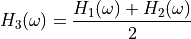
In the ”Trigger & FRF” Fig. 16 tab, one calculation type has to be chosen to define a modal test setup. The variables A and B stand for the complex spectra of the input (excitation) and output (response). Additionally, A’ and B’ present the complex conjugate spectra of the input and output channels.
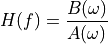
 Complex spectra of input channel.
 Complex spectra of output channel.
In case the output signal is noisy, the  algorithm can be used:

 Conjugate complex spectra of input channel
 Conjugate complex spectra of output channel
If the input signal is noisy, the  algorithm can be used:

In case both input and output signal are noisy,  or
or  can be used:

Coherence
The Coherence function compares the response function of the active group (excitation and response) with previously recorded response functions and returns values between 0 and 1. A value of 1 indicates an identical response function. Typically, measurements with a coherence below 0.8 are rejected and must be repeated.
Coherence calculation for two signals:

 Cross-spectral density
 and
and  Auto spectral density
Coherence calculation of a signal group and another signal:
![\gamma^{2}_{[A]B}(f) =
\frac
{G^{H}_{[A]B}(f) * G^{-1}_{[A][A]}(f) * G_{[A]B}(f)}
{G_{BB}(f)}](../_images/math/011c6f01319bdadeb6a3d3f4a51be8ea784d3041.png)
The following applies to this formula:
![\gamma^{2}_{[A]B}(f) \in [0,1]](../_images/math/04e566ee9d2e57afee09fdbcec7369521c35646b.png)
A value of 1 indicates a linear relationship between all signals in the selected group ![[a_{1}(t);\ldots;a_{n}(t)]](../_images/math/8e2171956e9140b92ae3a8821bc0fe3954b3ce7f.png) and the signal
and the signal  .
.
Whereas a value of 0 indicates no correlation between the signals  and .
and .
MIF - Mode Indicator functions
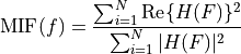
The Mode Indicator Function (MIF) evaluates the Frequency Response Function (FRF) of all excitation pathways. Values approaching 0 indicate the presence of a mode, while values approaching 1 indicate the absence of a mode. Additionally, the MIF for each excitation–FRF pair is calculated in the Excitation tab.
In the current implementation of the modal test, no model validation is implemented.
SDOF circle fit
The SDOF (Single Degree of Freedom) circle fit is a numerical method to estimate the natural frequency and loss factor. To calculate the loss factor, a spectral region, see Fig. 25 , is chosen where one natural frequency is assumed and transformed into a Nyquist plot, see Fig. 26 . In the Nyquist diagram, the point at which the circle crosses the Y-axis represents the exact natural frequency.
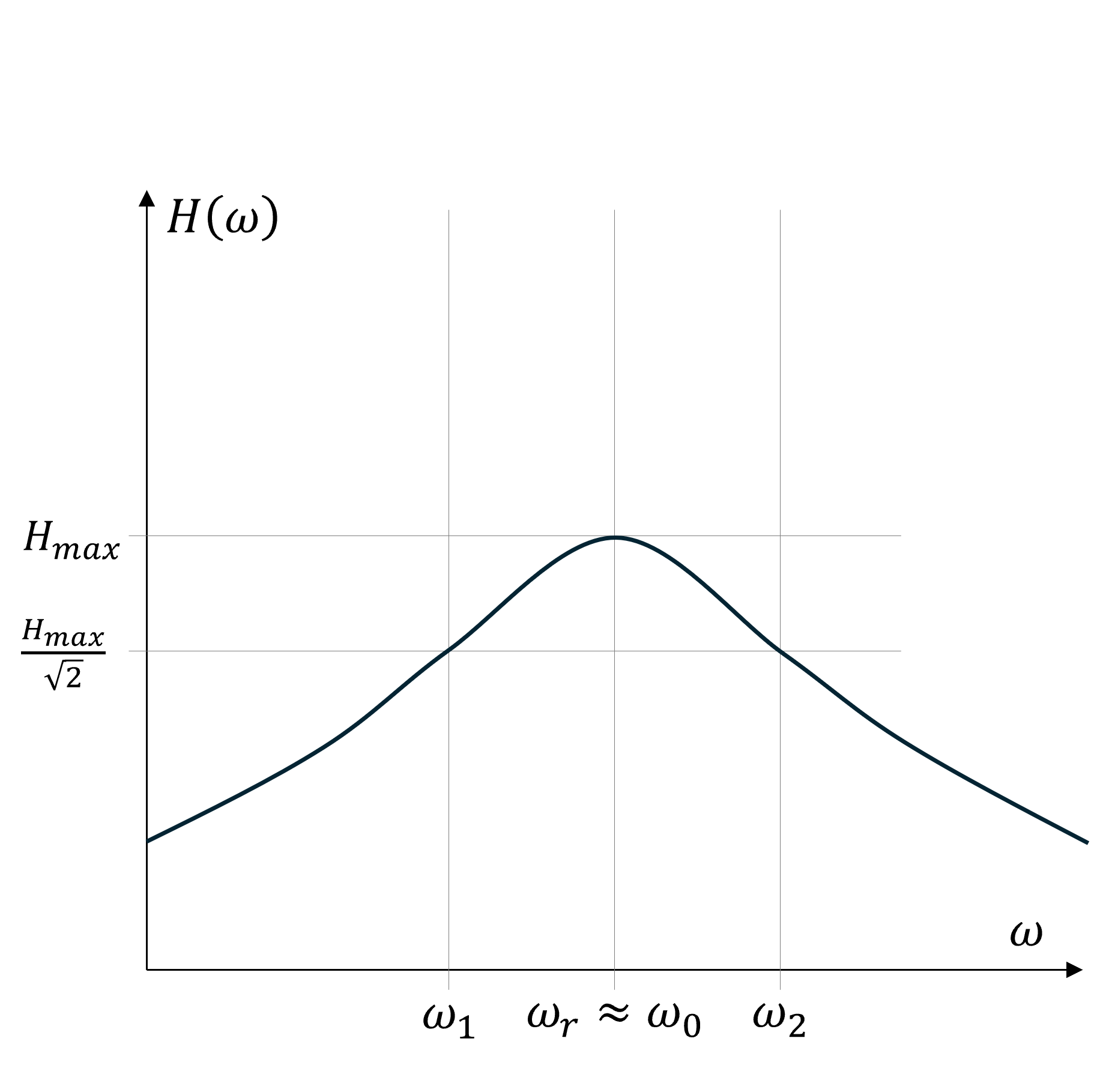
Fig. 25 Frequencies with the amplitude fit method using the amplitude response of an ideal single-mass oscillator
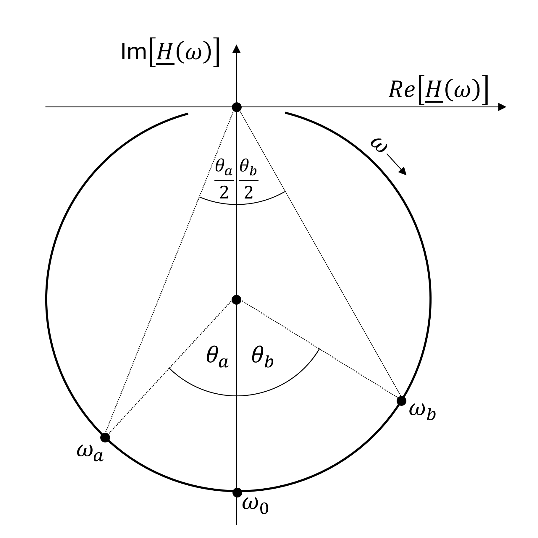
Fig. 26 Nyquist plot for SDOF with the locations of the natural frequency  and other frequencies
  and
and  

Subsequently, two known frequencies and their angle can be used to calculate the loss factor. The spectral region of interest must only contain one natural frequency.
![\eta
=
\frac{\omega_{0}^{2}-\omega_{b}^{2}}
{\omega_{0}^{2}\left[\tan\left(\frac{\theta}{2}\right)+\tan\left(\frac{\phi}{2}\right)\right]}
\approx
\frac{2(\omega_{a}-\omega_{b})}
{\omega_{0}\left[\tan\left(\frac{\theta}{2}\right)+\tan\left(\frac{\phi}{2}\right)\right]}](../_images/math/08930c5c33b7f16dfb2f46597a3ad40a950e27d1.png)
 Loss factor
Natural frequency (Eigenfrequenz)
Frequency above and
Frequency below the natural frequency
 Frequency response
An example of the OXYGEN implementation and application is shown in chapter SDOF circle fit .
Modal Test channel list – Recorded channels
In the current implementation of the modal test, the results of the Modal Test are divided into Excitation, Responses, and MIF (mode indicator function).
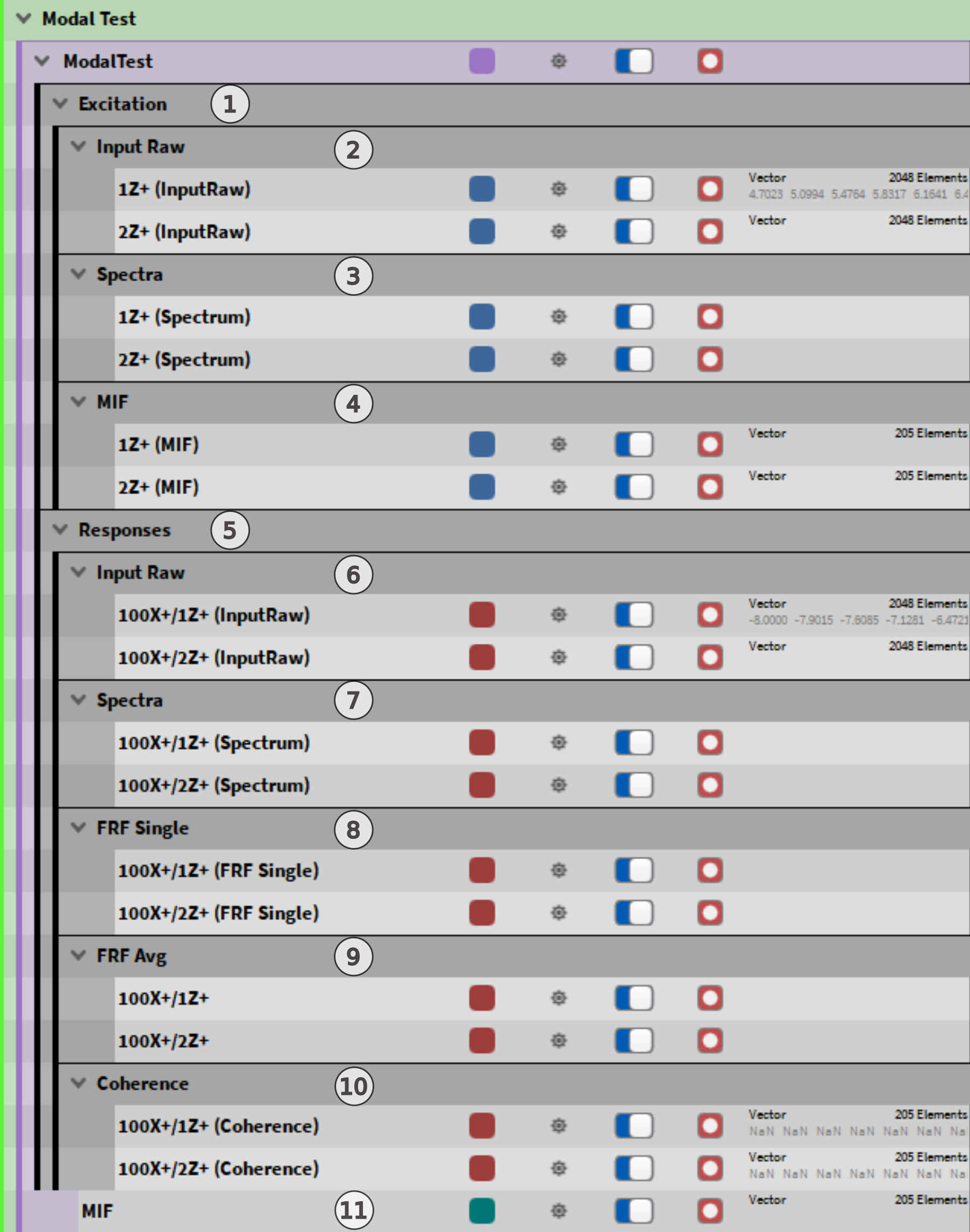
Fig. 27 Modal Test channel list
1 |
Excitation - grouping channel |
7 |
Spectra of input raw response channels |
2 |
Input Raw of excitation and response nodes |
8 |
FRF Single - FRF of single excitation event |
3 |
Spectra of input raw channels |
9 |
FRF AVG - Average of single FRFs |
4 |
MIF - calculated for each excitation node individually |
10 |
Coherence of excitation events |
5 |
Responses - grouping channel |
11 |
MIF - calculated over all excitation-FRF |
6 |
Input raw of excitation and response nodes |