Getting started
OXYGEN OPT-MODAL (OXYGEN MODAL) is the brand new modal test software option of DEWETRON’s OXYGEN measurement software that you can use with most DEWETRON hardware devices. In addition to the list of general features, this chapter describes how to perform the following tasks:
OXYGEN Basics
Setting up data channels
Creating a Modal Test setup
Navigating the Modal Test screen
Note
DEWETRON offers tailor-made product and application training to support you with your measurement and analysis. Please contact us for more information.
General Features
The following features enable a flexible and quick setup of a modal test for an arbitrary object.
Model Editor: Quick setup of a test object with excitation nodes and response nodes - Define measurement objects - Set the number of excitation/response points and general measurement axes and direction. This can be adjusted later in the “Measured Nodes”. - Define vertices - Set the position of excitation/response points in the coordinate system. - Define contour - Connect points by line, triangle, or quad operations in the 3D model. - Define measured nodes - Adjust measurement axes and directions including rotation.
Input Channels & Groups: Assignment of data channels to excitation modes and response - Drag and Drop response and excitation signals from the channel list - Automatically assign response signals from the channel list
Trigger & FRF: Setup of Triggers, FFT and FRF - Preview Excitation Amplitude and set trigger level - Define FFT sample size and maximum frequency - Set calculation type for frequency response function (H,H1,H2,H3, and Hv)
Modal Test Screen: Intuitive visualization of excitation events - Amplitude - Response/Excitation (e.g. g/N or m/s²/N) - FRF Single - Data of single trigger event in amplitude plot - Phase shift - Response/Excitation [°] - Coherence - Response/Excitation [1..0] - MIF - Mode indicator function in coherence plot - Warnings - Custom range limit, measurement range exceeded, double hit
In addition to the great measurement functions of OXYGEN, the MODAL-Option enables the recording of the following excitation and response characteristics.
Excitation - Input Raw (Raw input values for each excitation point) - Spectra (Spectrum of each excitation)
Responses - Input Raw (Raw input values for each measurement point per excitation) - Spectra (Spectrum of each measurement point per excitation) - FRF Single (Frequency response function for each triggered measurement) - FRF Average (Frequency response function for the average of triggered measurement) - Coherence (Similarity of each excitation and response)
MIF (Mode indicator function)
Note
The requirements for full functionality and maximum speed are: - CPU: Intel Core i5 3rd Generation or better - RAM: 8 GB or greater - DAQ: TRION - OS: Windows 7 64 Bit or newer (Linux Version on request) - Preinstalled DAQ driver (TRION API)
OXYGEN Basics
Turn on your DEWETRON measurement device
Use the provited DEWETRON OXYGEN (R7.0 or higher) Installer if not installed already.
Start the OXYGEN measurement software (if not launched automatically)
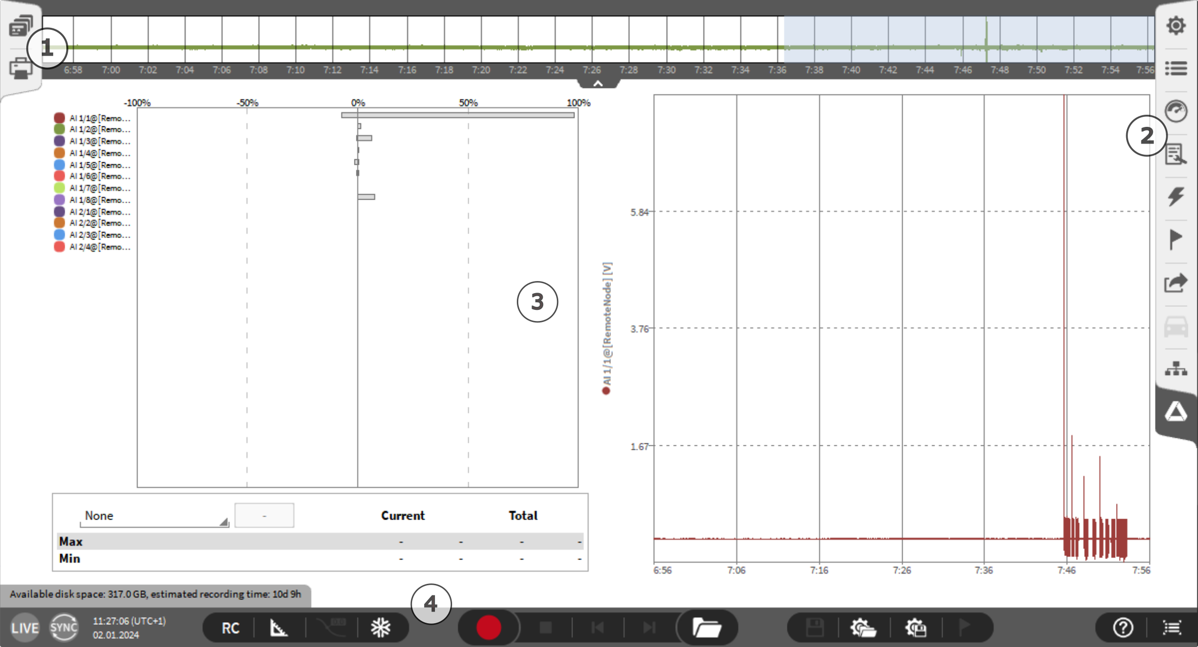
Fig. 1 Startup screen
Legend
① Screens and Reporting ② Menu Bar ③ Instrument area ④ Action bar
The Startup screen contains four main areas, the ① “Screens and Reporting” tabs, where additional screens can be added and reports can be created. The ② “Menu bar” contains a variety of functionalities including the measurement settings, the data channel list, and the measurement instruments, which can be added to the instrument area ③ by drag and drop. By default, a saturation meter on the left and a chart recorder on the right are placed in the instrument area. The fourth area ④ is the “Action bar”, where the measurement can be controlled and the setup saved or loaded.

Fig. 2 Action Bar
5 |
Instrument state indicator |
13 |
Jump forward |
6 |
Screen lock |
14 |
Open data file for analysis (.dmd) |
7 |
Design mode |
15 |
Save changes in data file (Play Mode) |
8 |
Activate/Deactivate cursor for active instrument |
16 |
Open configuration setup (.dms) |
9 |
Freeze screen content |
17 |
Save configuration setup (.dms) |
10 |
Start recording / arm trigger |
18 |
Insert marker during recording |
11 |
Stop recording |
19 |
GUI tutorial |
12 |
Jump backward |
20 |
Open/Close channel list |

Fig. 3 Menu Bar
21 |
Open measurement settings |
26 |
Open event list |
22 |
Open channel list |
27 |
Open export settings |
23 |
Open instruments panel |
28 |
Open network and sync menu |
24 |
Open instrument properties |
29 |
Open birds eye |
25 |
Open trigger events |
30 |
Open OXYGEN setup |
For further infotrmation, please see the latest OXYGEN manual in our Customer Care Center: https://ccc.dewetron.com/pl/oxygen.
Setting up data channels
- The first step after switching on your DEWETRON measurement device is to set up your data channels in the channel list.
Switch to the channel list ①
Click on the channel setup ② (gear icon)
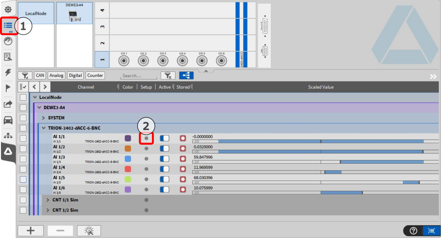
Fig. 4 Channel setup in channel list
Proper measurements require correct sensor scaling. In most cases, the sensor label gives information about the input/output scaling. This value often known as the “transducer factor”, “ratio” or “sensitivity”. Important is the unit of the scaling, e.g 100.59 mV/g or 10.257 mV/(m/s²).
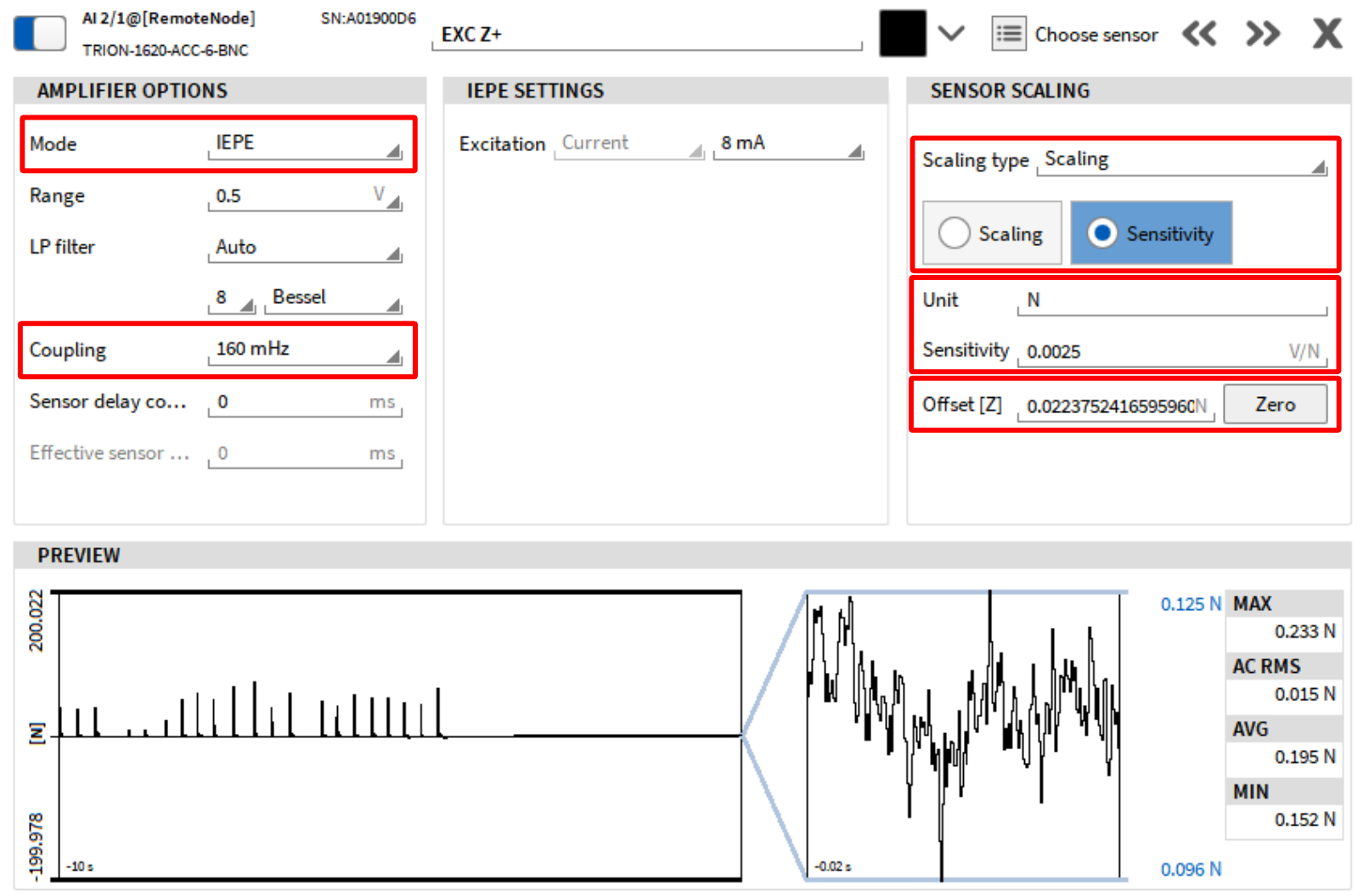
Fig. 5 IEPE Sensor scaling
Select the mode fitting your sensor (e.g. IEPE).
Select the type of scaling/sensitivity.
Define your unit and the scaling/sensitivity.
Select coupling mode (high-pass filter) to reduce noise and drift.
Optionally zero your offset.
Creating a Modal Test
To create a Modal Test, go to the channel list and use the (+) button ① on the bottom left of the channel list to add “Modal Test”, found in the “Advanced Math” category. This adds the Modal Test Channel ② in the channel list and the Modal Test tab ③ right above the OXYGEN setup tab and forwards you to the Model Editor (see Fig. 9 ).
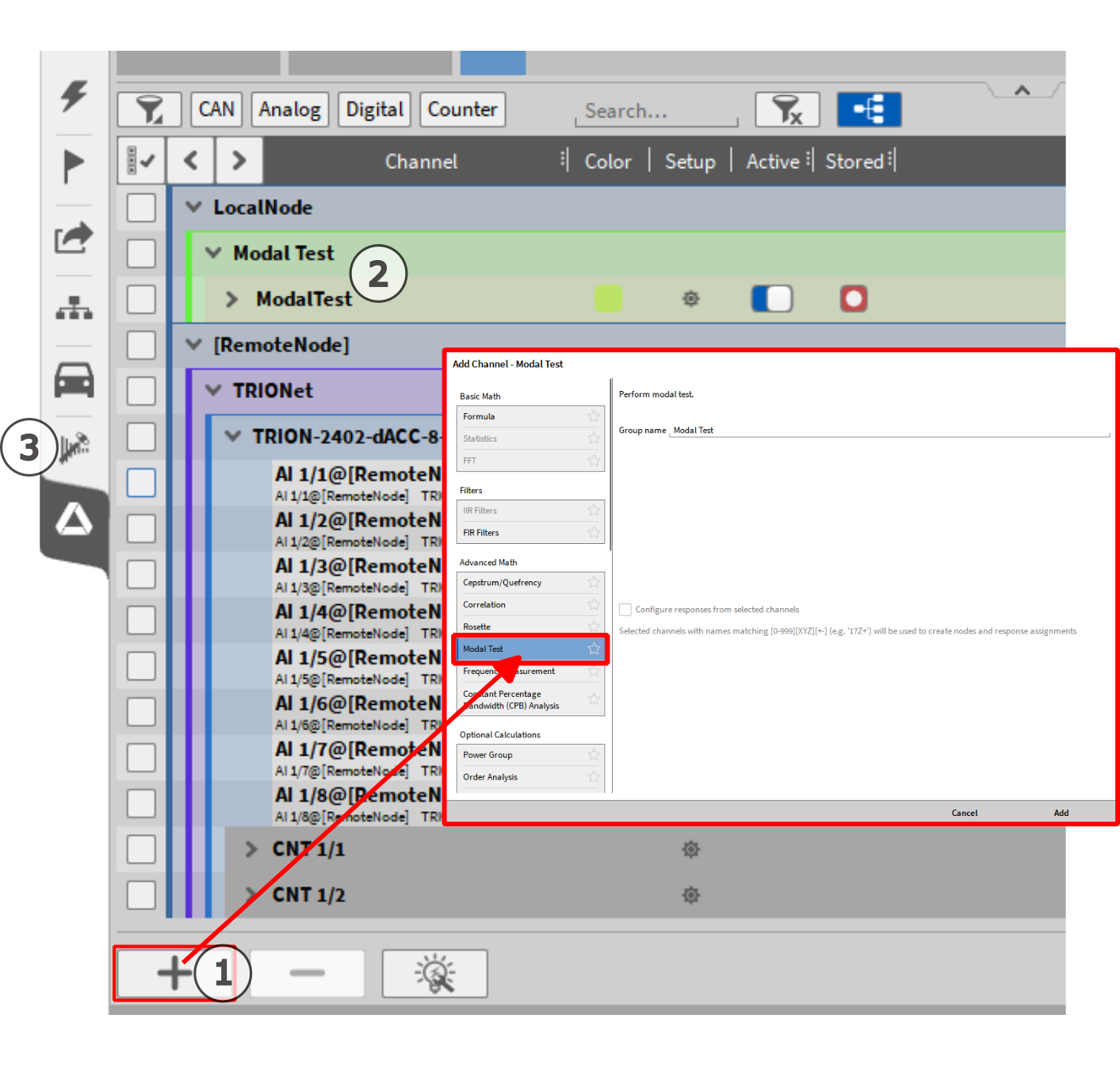
Fig. 6 Set up Modal test channel
Legend
① Add Modal Test Group ② Modal Test channel ③ Modal Test Tab
The next page describes an alternative method, which utilizes selected channels to create a test object, In case you didn´t select channels for the Modal Test setup, skip to the definition of the test object in the Modal Editor in Fig. 9 .
Alternatively, if the respective channels match the naming convention “[0-999][XYZ][+-]”, they can be used to create a test object. The tick in the checkbox indicates if the naming is correct. After clicking “Add” the “Model Editor” is opened, which can also be accessed by clicking/swiping the Modal Test tab.
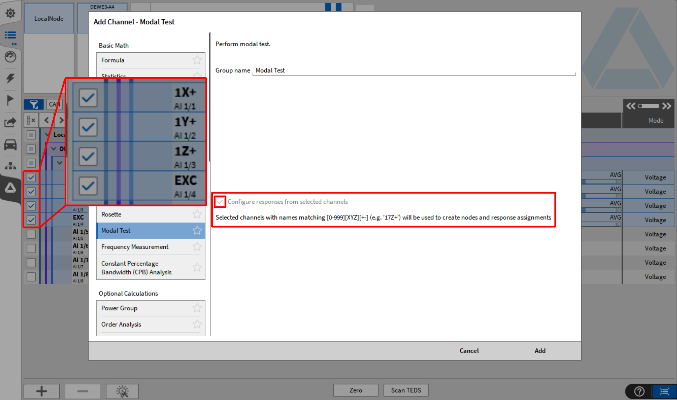
Fig. 7 Use channels for test object setup
Fig. 7 shows the Model Editor alreay populated with a generated test object, based on the selected channels for excitation and response nodes. The test object can be further edited as described in the next pages.
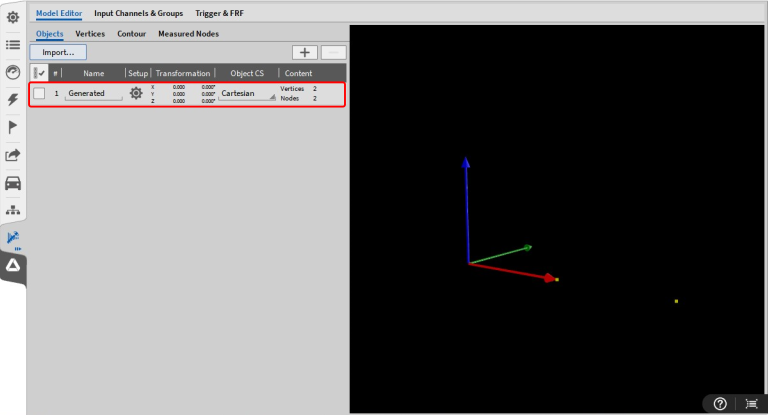
Fig. 8 Predefined Model Editor
When creating a Modal Test without selected channels, the Model Editor tab is empty. It can also be opened by clicking or swiping the Modal Test tab ①. The Model Editor ② is the first of three tabs to define the Modal Test setup. First you need to set the number of excitation points and button ③. Further settings for the test object can be changed in the sub-tabs of the Model Editor vertices, Contour, and Measured Nodes ④.
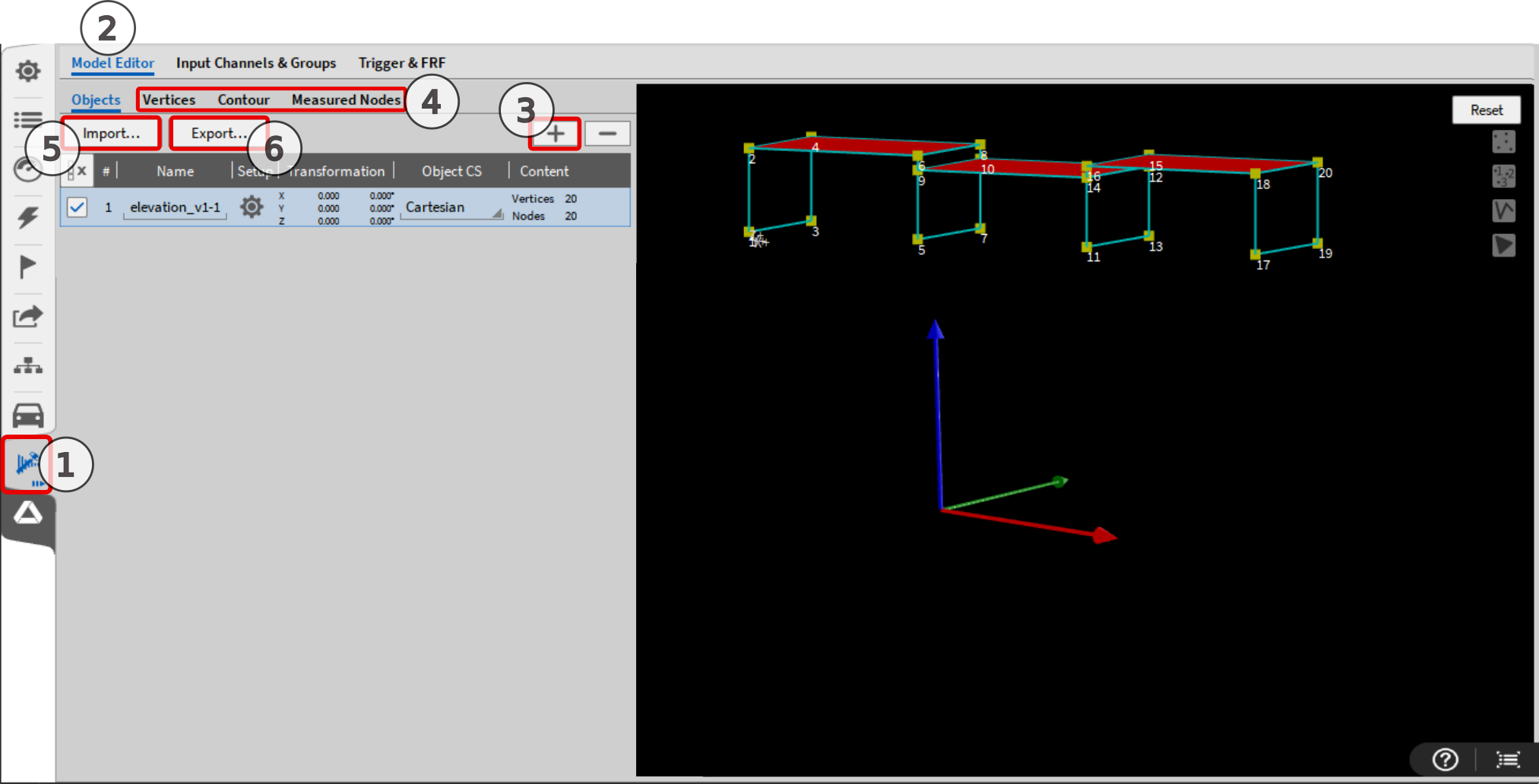
Fig. 9 Model Editor
Attention
The current implementation supports the import ⑤ and export ⑥ of a test object via a geometry file in the *.unv or *.uff format.
After pressing the (+) button in the Model Editor to add a test object, the following window pops up. Here the number of excitation nodes (usually up to 12) and the number of response nodes (usually up to 12) are defined in addition to the overall response directions. The axes of excitation/s and response nodes can be edited in the “Measured Nodes” tab. Note that the number of response nodes stands for the number of points at which a response is measured and not for the number of total response signals. For example, one response node can have 3 axes that are measured and provide 3 data channels, since all are measured at one point they count as one response node.
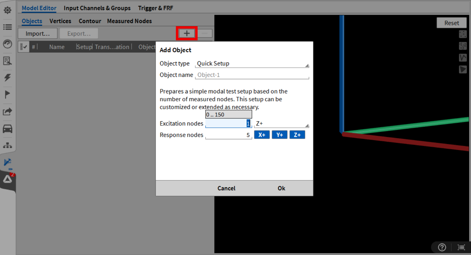
Fig. 10 Add Test Object
If needed, the excitation and response axes can be modified in the “Measured Nodes” tab. In Fig. 11 , two excitation points and one response positions with three directions is defined. The response nodes can be to mono-, bi, or triaxial in the positive or negative direction.
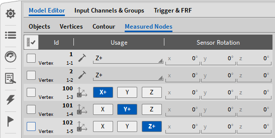
Fig. 11 Model Editor - Measured Nodes
To add/remove nodes of the test object, switch to the “Vertices” tab and use the (+) or (-) buttons ①. When a new node is created ② (node 1-4), the type (excitation or response) can be defined by selecting the hammer icon (excitation) ③ or the axes icon (response nodes) ④.
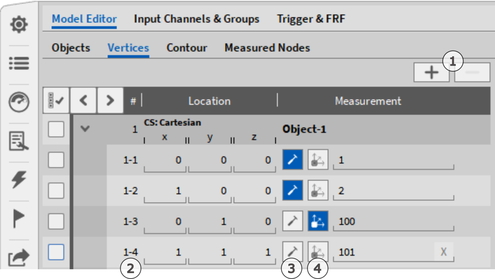
Fig. 12 Add/Remove nodes
In the next Fig. 13 , the new node was defined as a response node. To change the type of coordinates from Cartesian to Cylindrical, switch to the “Objects” tab.
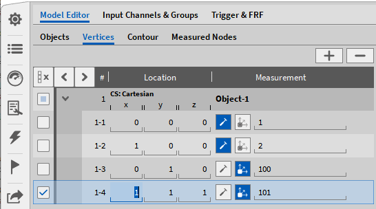
Fig. 13 New response node
The defined response nodes can be connected by a custom contour, which can be set in the “Contour” tab. Simply use the naming (1-4, number of test object - number of signal channel), as defined in the “Vertices” tab, and choose the type of connenction (line ①, triangle ② or quad ③).
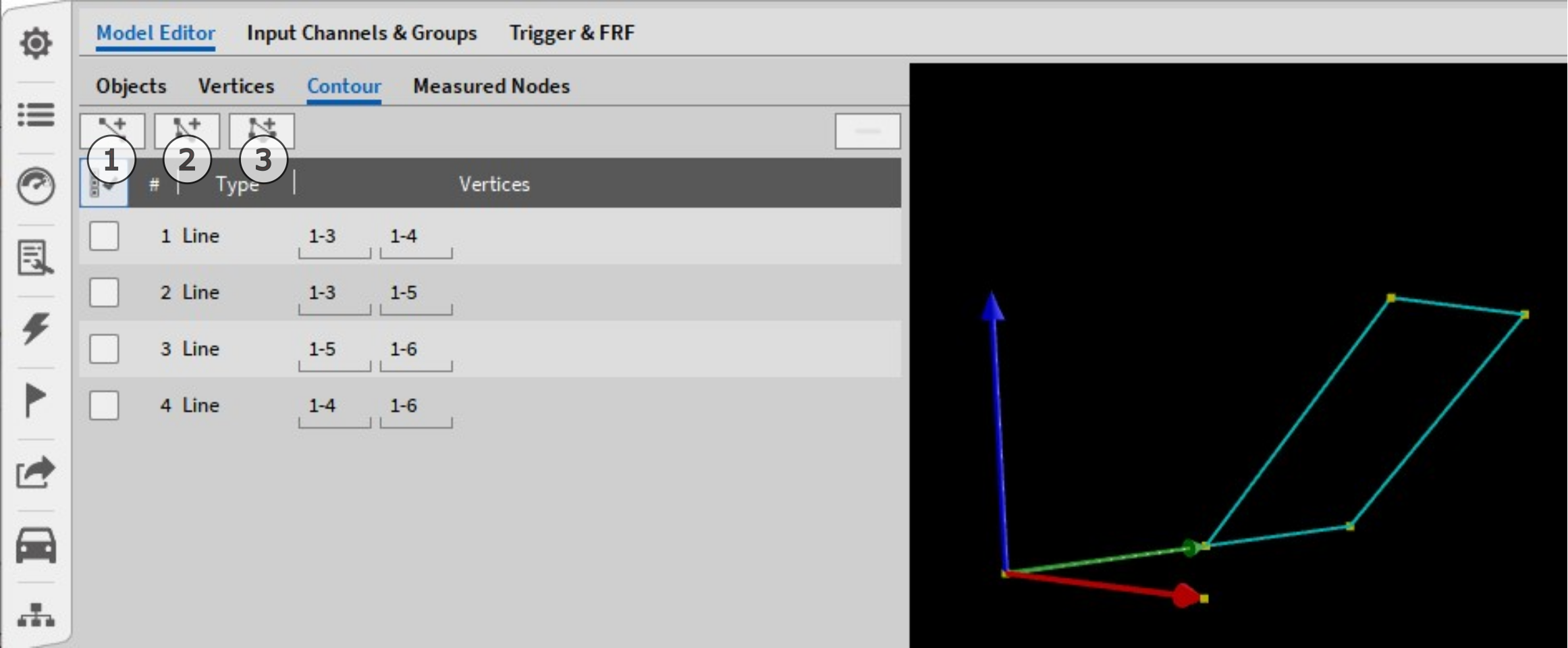
Fig. 14 Test Object Contour
The next step after setting up a test object, is to define the input channels in the second tab “Input Channels & Groups”. Here the excitation channel can be added by drag and drop ①, while the response channels can be drag and dropped ② or “Auto assigned” ③, which automatically adds them to the selection sequence to undefined response groups. The channel list shows all available data channels regardless of their type.
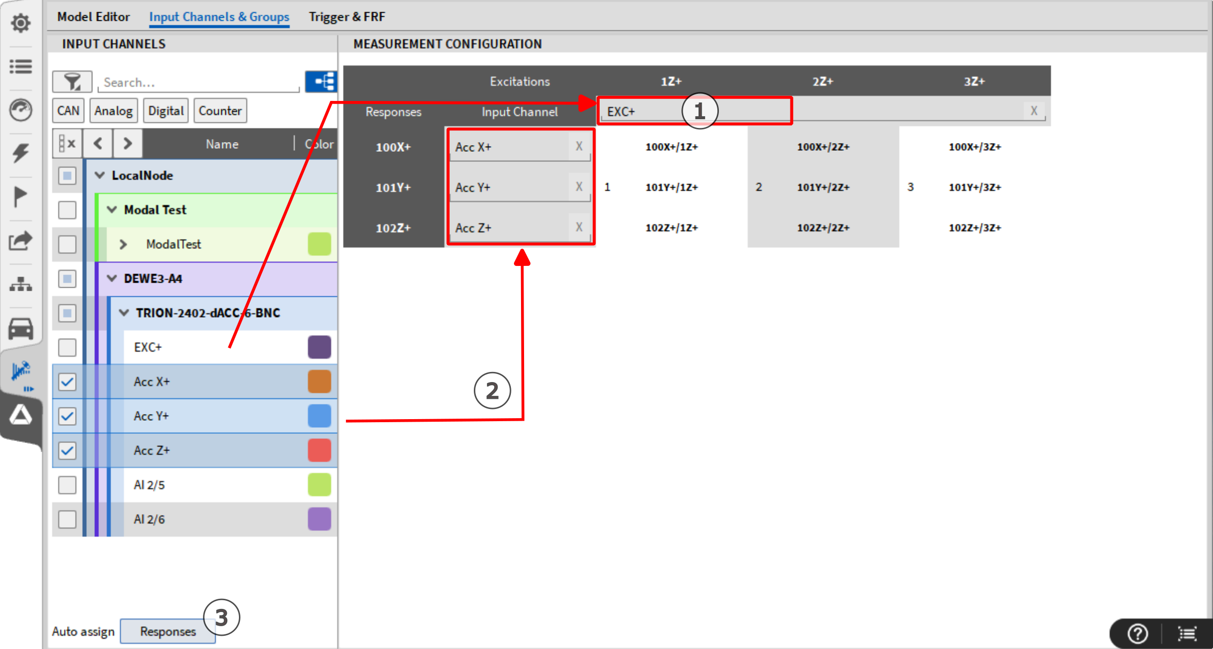
Fig. 15 Input Channel & Groups
The third and last tab to define the Modal Test setup is the “Trigger & FRF” menu, where the trigger can be set based on an excitation and response preview. In the Trigger section, the “Required triggers per group” ① is used to define how many excitation events are averaged for one excitation point. The correct “Trigger level” ② can be set by using the preview window ②, which can be auto-scaled by a click on its label. If the check box “Second hit level” ③ is ticked, signals higher than x% of the trigger peak lead to a warning in the of a pink color and an exclamation mark of the respective excitation bar. The “Warning level” ④ can be set to detect excitation even74ts that exceed a percentage of the range. For recording the spectrum, the “Pretrigger” ⑤ sets the percentage of samples to include, before the trigger level is reached. The configuration for the FFT calculation is done in the FFT section ⑥, which enables to setting of a data size, a line resolution, and a maximum frequency. For further information on the FFT calculation see the OXYGEN manual . The maximum frequency should be set to 1/10th of the sample rate, for example to a maximum frequency of 1000 Hz for a sample rate of 10kHz. The last setting of this tab is the FRF (frequency response function) “Type” ⑦ which is used to set the calculation type. The formulas for the FRF are described from formula 2.1 to formula 2.5. The two preview windows on the left ⑧ show the live signal of the excitation and response nodes, while the two windows on the right ⑨ display the last recorded trigger event.
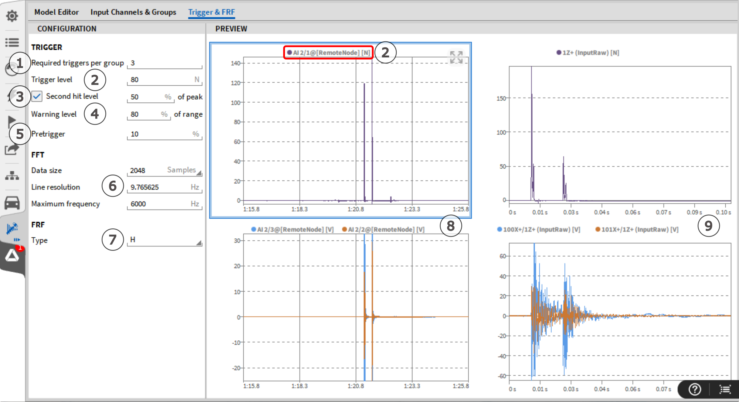
Fig. 16 Trigger & FRF
If clicking on the label to auto-scale, has no effect, the design mode might be still enabled. To deactivate, simply double-click on the instrument and disable the blue triangle button.
Fig. 17 Design mode
The Modal Test screen
On the measurement screen, the modal test screen can be added for visualization, recording and navigation of the modal test. To create this screen click on the “Create Modal Screen” button ①, see Fig. 18 . This screen always displays the data of the active excitation group ⑥. The following items ① - ⑰ can be found in Fig. 18 .
1 |
Create Modal Test Screen: Creates a new screen based on a Modal Test template. |
10 |
Spectra of excitation channel (FFT) |
2 |
Active: Deactivates FRF calculation i.e. in case sensors are changed. |
11 |
Live data of response channels |
3 |
Reject: Deletes the last hit(s) successively. |
12 |
Recorded signal of response channels |
4 |
Single: Shows data of actual hit in Amplitude FRF and Bode Plot. |
13 |
Spectra of response channels (FFT) |
5 |
MIF: Display the mode indicator function in the coherence banner. |
14 |
Amplitude response: Spectrum of amplitude ratio between response and excitation |
6 |
Select/show the currently active group to measure/view/discard. |
15 |
Phase shift response: Spectrum of phase shift between response and excitation [°] |
7 |
Shows the saturation and progress of the latest measurement group. Switch between single hits of the currently selected group. |
16 |
Coherence function: Similarity between excitation and response of recorded events |
8 |
Live data of excitation channel. |
17 |
Modal Shape animation: Animation of the modal test object for a specific frequency. See Fig. 18 for detailed usage. |
9 |
Recorded signal of excitation channel |
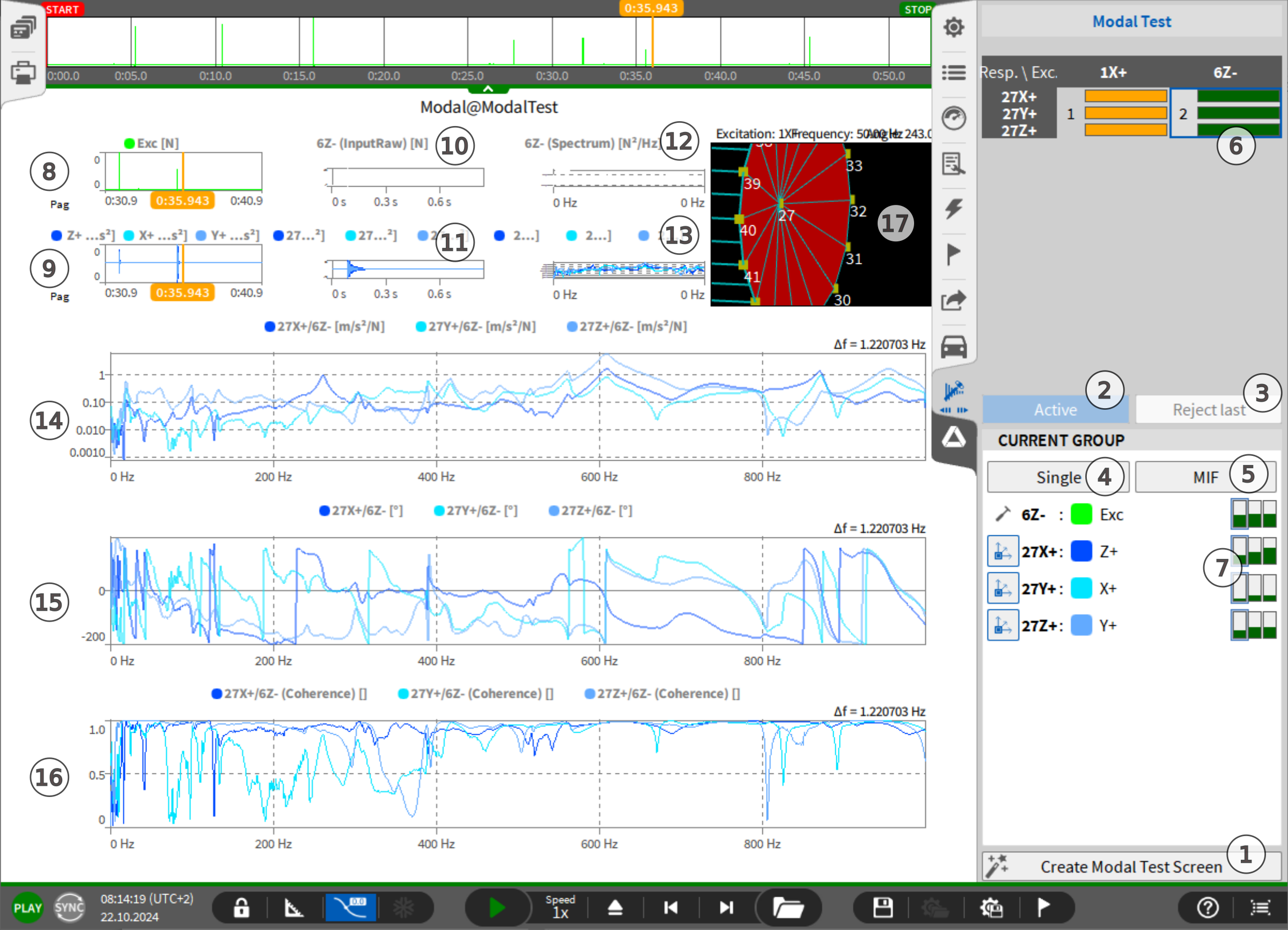
Fig. 18 Modal Test Screen Overview
A standard measurement procedure proceeds as follows: The trigger button ② is active by default. If not, set the button to active and excite the test object. As a result, the bar indicator ⑦ should be filled, in this case, three times with a green color. To repeat an excitation event and discard the last one, the (Reject last) button ③ can be used. To switch to previous excitation groups, the desired excitation group ⑥ can be clicked to set it as the active group and display its data. To further analyze the data, a single FRF can be displayed in the amplitude response ⑭ by clicking ④ . Furthermore, the MIF can be added to the coherence spectrum ⑯ by clicking ⑤ . For more details about the MIF calculation go to formula 2.8 and for the Coherence calculation, to formula 2.6 and formula 2.7. Each instrument can be modified to change the displayed data, for example, the amplitude response can be set to display the real or imaginary part instead. Just click on the instrument to be edited and click the instrument properties tab seen in the next Fig. 20 ① to choose the desired data. For more information on the spectrum analyzer, see the OXYGEN manual .
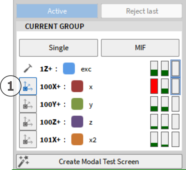
Fig. 19 Selection of response group
The individual response groups can be hidden, shown in Fig. 19 ① where a click on the axes symbol toggles the displayed data in the amplitude response, seen in figure 1.18 ⑭ , the phase shift response ⑮ and the coherence function ⑯ . In the first excitation of this group, the x response bar is displayed as red. This indicates an exceeding of the sensor range. Further details are described in the operation basics chapter.
The data displayed in the modal test screen instruments can be further customized. For example the bode diagram can be changed to show real part of the vibration instead of the amplitude. To revert to the default template, just click again on the ”Create Modal Test Screen” button ① in Fig. 18 , which adds a new screen based on the default modal test screen template. To further edit the modal test screen, the instrument group can be dismantled and changed to the preferred instruments. Click on the modal test group followed by clicking on dismantle ② in the properties.
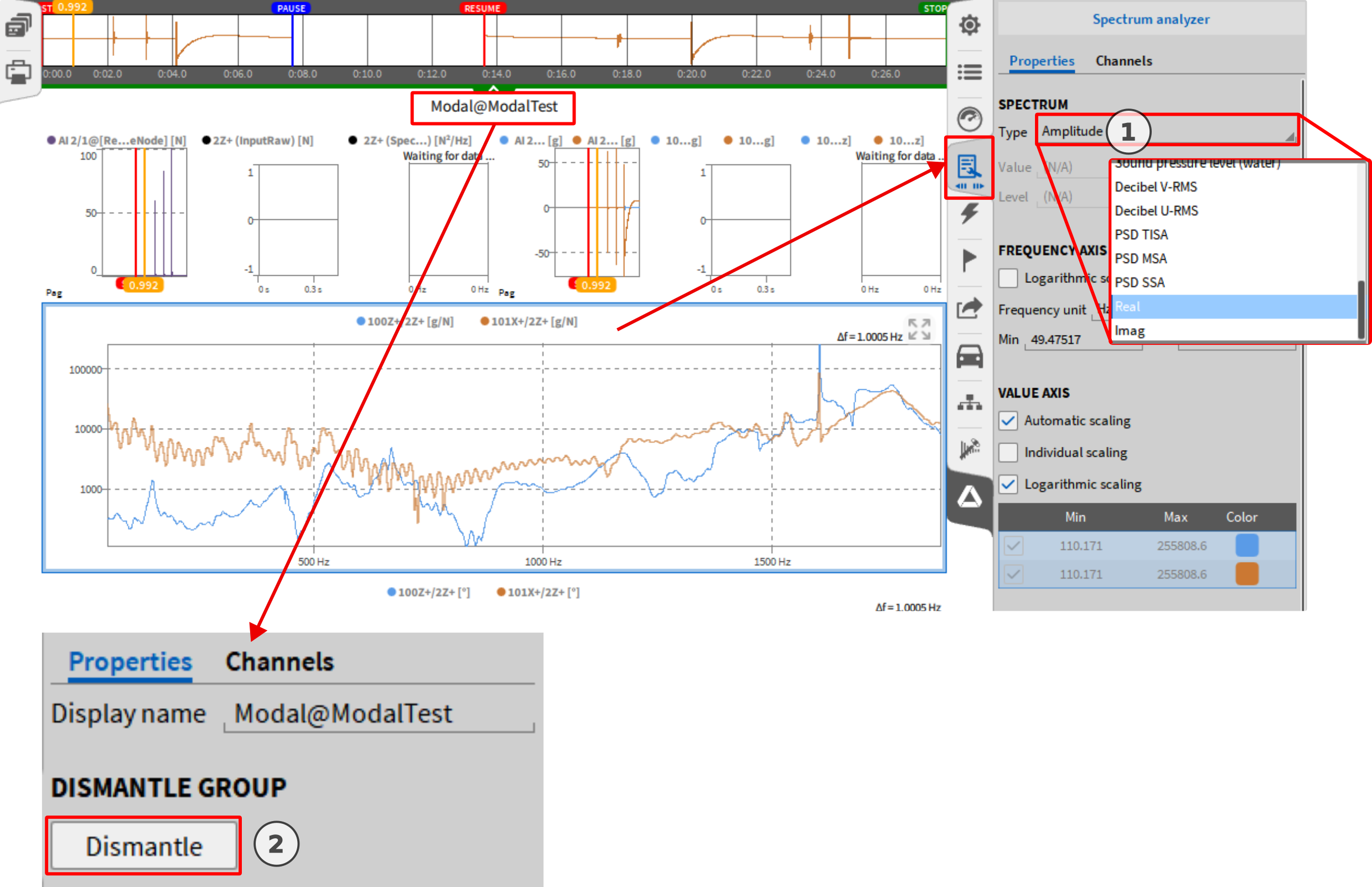
Fig. 20 Instrument properties and dismantling template
Modal Shape animation
The modal shape animation instrument can be found in the instruments list in the miscellaneous tab and is by default included in the modal test screen. It has the following features in the instrument properties:
① Set the excitation point, whereas ”Auto” selects the first recorded excitation point.
② The animated frequency can be selected either manually or based on an adjacent instrument or an instruments on the page. To select a frequency based on an adjacent/page instrument, choose the respective mode and click via cross hair into the bode plot. This will make a cursor line appear which specifies the frequency for the modal shape animation. To manually specify the frequency, set the dropdown to ”Manually specified” and use the slider or the text box.
③ Deflection controls the animation speed, the amplitude of the oscillation and the replay of the animation which loops the selected excitation event. With MAX (+) the largest deflection and with (-) the smallest deflection is shown.
④ View can hide part of the model object and resets the zoom and position of the model object.
⑤ Export a video of the instrument (modal shape animation) or entire screen for reporting purposes. The export is only available in PLAY mode and the video format is *.mkv. The number of animation cycles can be defined from 1 to 10.
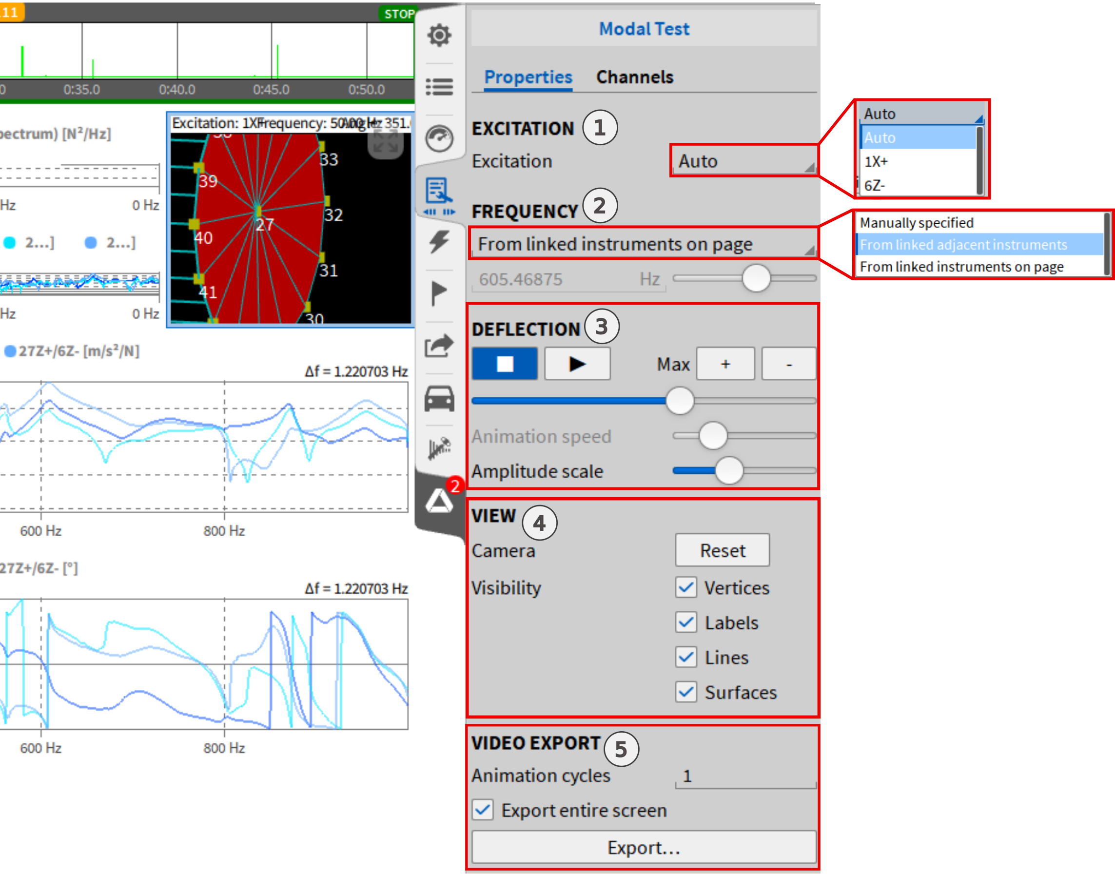
Fig. 21 Modal Shape animation instrument
SDOF circle fit
The SDOF Circle Fit can estimate the damping in simple structural systems, characterized by well-separated, non-overlapping modes. These systems can be effectively analyzed as individual Single Degree Of Freedom (SDOF) systems, enabling accurate damping estimation. The application of this method is illustrated in the example Frequency Response Function (FRF) graph provided below, which demonstrates the distinct modal characteristics of such simple structures. First choose the Nyquist instrument from the instruments panel or open the nyquist template, in the bottom of the screens menu, which is available after creating a modal test.
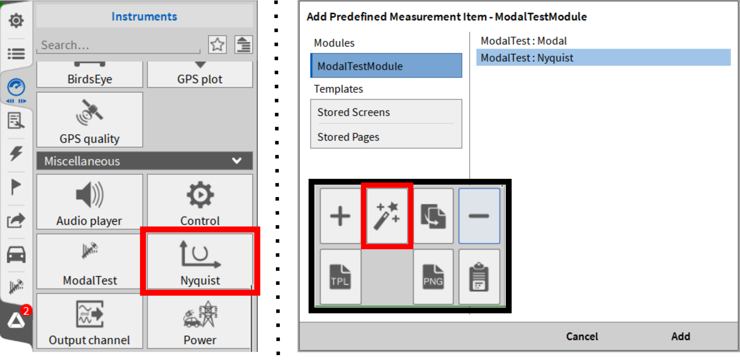
Fig. 22 Nyquist instrument
When choosing the Nyquist template, the FRF averages of the first excitation event are automatically assigned to a spectrum analyzer instrument and the Nyquist instrument. The first step is to determine if a manual frequency range or a frequency range based on another instrument on the page or nearby should be used for the circle fit. To choose the frequency bandwidth with another instrument, the spectrum analyzer, three options are available.
Single cursor - Select the center frequency with one cursor, whereas 10 bins below and above the chosen frequency are used as default for the circle fit. This is also the case if the frequency is chosen manually.
Dual cursor - Select the frequency range of interest with upper and lower cursor. The center frequency is automatically calculated as middle of the selected band.
Triple cursor - Select the lower, middle and upper frequency to specify an asymmetrical frequency range.
This means if a Bode plot is linked, one two or three cursors can be set to specify the frequency band of the Nyquist plot. See the example Fig. 23 which facilitates a single cursor in an amplitude Bode plot.
In this example the frequency range ① is chosen via the amplitude bode plot ② on the same page and the fitting parameter is calculated by center and radius ③ . There is also the option to only calculate the loss factor via the center or just display the Imaginary and Real part of the signal. In ④ the resulting fitting parameter(Natural frequency and Loss factor) as displayed and can be copied to the clipboard.
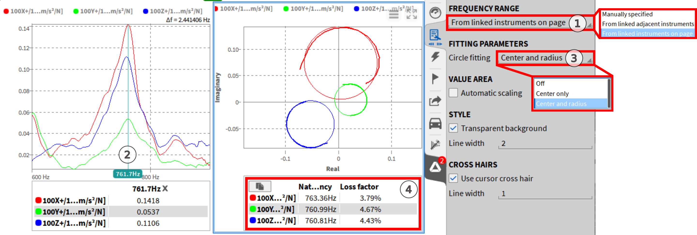
Fig. 23 SDOF circle fit
More information regarding the calculation basis and theory of the circle fit can be found at chapter SDOF circle fit .